The CIFAR-10 small photo classification problem is a standard dataset used in computer vision and deep learning.
Although the dataset is effectively solved, it can be used as the basis for learning and practicing how to develop, evaluate, and use convolutional deep learning neural networks for image classification from scratch.
This includes how to develop a robust test harness for estimating the performance of the model, how to explore improvements to the model, and how to save the model and later load it to make predictions on new data.
In this tutorial, you will discover how to develop a convolutional neural network model from scratch for object photo classification.
After completing this tutorial, you will know:
- How to develop a test harness to develop a robust evaluation of a model and establish a baseline of performance for a classification task.
- How to explore extensions to a baseline model to improve learning and model capacity.
- How to develop a finalized model, evaluate the performance of the final model, and use it to make predictions on new images.
Let’s get started.

How to Develop a Convolutional Neural Network From Scratch for CIFAR-10 Photo Classification
Photo by Rose Dlhopolsky, some rights reserved.
Tutorial Overview
This tutorial is divided into six parts; they are:
- CIFAR-10 Photo Classification Dataset
- Model Evaluation Test Harness
- How to Develop a Baseline Model
- How to Develop an Improved Model
- How to Develop Further Improvements
- How to Finalize the Model and Make Predictions
Want Results with Deep Learning for Computer Vision?
Take my free 7-day email crash course now (with sample code).
Click to sign-up and also get a free PDF Ebook version of the course.
CIFAR-10 Photo Classification Dataset
CIFAR is an acronym that stands for the Canadian Institute For Advanced Research and the CIFAR-10 dataset was developed along with the CIFAR-100 dataset by researchers at the CIFAR institute.
The dataset is comprised of 60,000 32×32 pixel color photographs of objects from 10 classes, such as frogs, birds, cats, ships, etc. The class labels and their standard associated integer values are listed below.
- 0: airplane
- 1: automobile
- 2: bird
- 3: cat
- 4: deer
- 5: dog
- 6: frog
- 7: horse
- 8: ship
- 9: truck
These are very small images, much smaller than a typical photograph, and the dataset was intended for computer vision research.
CIFAR-10 is a well-understood dataset and widely used for benchmarking computer vision algorithms in the field of machine learning. The problem is “solved.” It is relatively straightforward to achieve 80% classification accuracy. Top performance on the problem is achieved by deep learning convolutional neural networks with a classification accuracy above 90% on the test dataset.
The example below loads the CIFAR-10 dataset using the Keras API and creates a plot of the first nine images in the training dataset.
# example of loading the cifar10 dataset
from matplotlib import pyplot
from keras.datasets import cifar10
# load dataset
(trainX, trainy), (testX, testy) = cifar10.load_data()
# summarize loaded dataset
print('Train: X=%s, y=%s' % (trainX.shape, trainy.shape))
print('Test: X=%s, y=%s' % (testX.shape, testy.shape))
# plot first few images
for i in range(9):
        # define subplot
        pyplot.subplot(330 + 1 + i)
        # plot raw pixel data
        pyplot.imshow(trainX[i])
# show the figure
pyplot.show()
Running the example loads the CIFAR-10 train and test dataset and prints their shape.
We can see that there are 50,000 examples in the training dataset and 10,000 in the test dataset and that images are indeed square with 32×32 pixels and color, with three channels.
Train: X=(50000, 32, 32, 3), y=(50000, 1)
Test: X=(10000, 32, 32, 3), y=(10000, 1)
A plot of the first nine images in the dataset is also created. It is clear that the images are indeed very small compared to modern photographs; it can be challenging to see what exactly is represented in some of the images given the extremely low resolution.
This low resolution is likely the cause of the limited performance that top-of-the-line algorithms are able to achieve on the dataset.
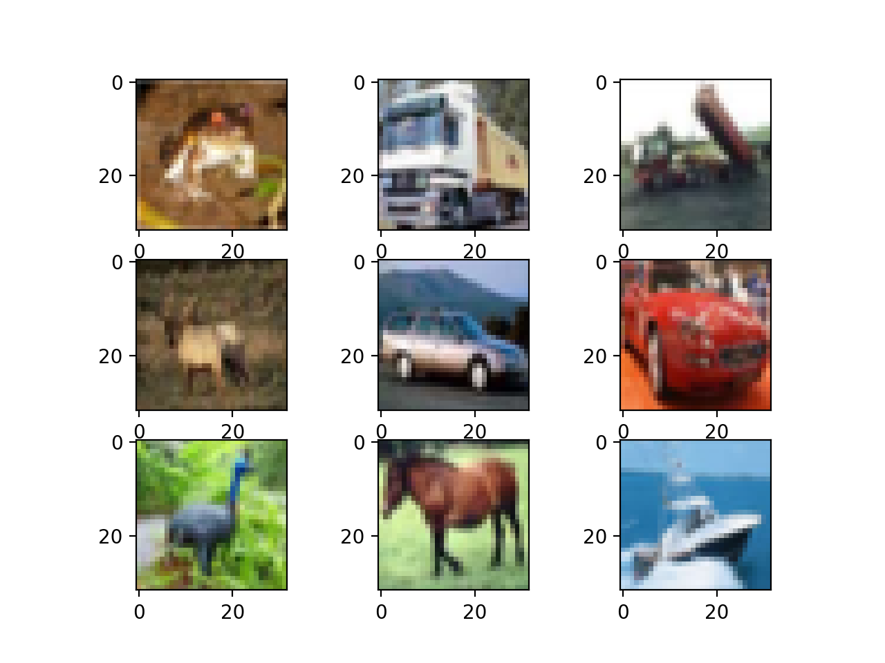
Plot of a Subset of Images From the CIFAR-10 Dataset
Model Evaluation Test Harness
The CIFAR-10 dataset can be a useful starting point for developing and practicing a methodology for solving image classification problems using convolutional neural networks.
Instead of reviewing the literature on well-performing models on the dataset, we can develop a new model from scratch.
The dataset already has a well-defined train and test dataset that we will use. An alternative might be to perform k-fold cross-validation with a k=5 or k=10. This is desirable if there are sufficient resources. In this case, and in the interest of ensuring the examples in this tutorial execute in a reasonable time, we will not use k-fold cross-validation.
The design of the test harness is modular, and we can develop a separate function for each piece. This allows a given aspect of the test harness to be modified or interchanged, if we desire, separately from the rest.
We can develop this test harness with five key elements. They are the loading of the dataset, the preparation of the dataset, the definition of the model, the evaluation of the model, and the presentation of results.
Load Dataset
We know some things about the dataset.
For example, we know that the images are all pre-segmented (e.g. each image contains a single object), that the images all have the same square size of 32×32 pixels, and that the images are color. Therefore, we can load the images and use them for modeling almost immediately.
# load dataset
(trainX, trainY), (testX, testY) = cifar10.load_data()
We also know that there are 10 classes and that classes are represented as unique integers.
We can, therefore, use a one hot encoding for the class element of each sample, transforming the integer into a 10 element binary vector with a 1 for the index of the class value. We can achieve this with the to_categorical() utility function.
# one hot encode target values
trainY = to_categorical(trainY)
testY = to_categorical(testY)
The load_dataset() function implements these behaviors and can be used to load the dataset.
# load train and test dataset
def load_dataset():
        # load dataset
        (trainX, trainY), (testX, testY) = cifar10.load_data()
        # one hot encode target values
        trainY = to_categorical(trainY)
        testY = to_categorical(testY)
        return trainX, trainY, testX, testY
Prepare Pixel Data
We know that the pixel values for each image in the dataset are unsigned integers in the range between no color and full color, or 0 and 255.
We do not know the best way to scale the pixel values for modeling, but we know that some scaling will be required.
A good starting point is to normalize the pixel values, e.g. rescale them to the range [0,1]. This involves first converting the data type from unsigned integers to floats, then dividing the pixel values by the maximum value.
# convert from integers to floats
train_norm = train.astype('float32')
test_norm = test.astype('float32')
# normalize to range 0-1
train_norm = train_norm / 255.0
test_norm = test_norm / 255.0
The prep_pixels() function below implement these behaviors and is provided with the pixel values for both the train and test datasets that will need to be scaled.
# scale pixels
def prep_pixels(train, test):
        # convert from integers to floats
        train_norm = train.astype('float32')
        test_norm = test.astype('float32')
        # normalize to range 0-1
        train_norm = train_norm / 255.0
        test_norm = test_norm / 255.0
        # return normalized images
        return train_norm, test_norm
This function must be called to prepare the pixel values prior to any modeling.
Define Model
Next, we need a way to a neural network model.
The define_model() function below will define and return this model and can be filled-in or replaced for a given model configuration that we wish to evaluate later.
# define cnn model
def define_model():
        model = Sequential()
        # ...
        return model
Evaluate Model
After the model is defined, we need to fit and evaluate it.
Fitting the model will require that the number of training epochs and batch size to be specified. We will use a generic 100 training epochs for now and a modest batch size of 64.
It is better to use a separate validation dataset, e.g. by splitting the train dataset into train and validation sets. We will not split the data in this case, and instead use the test dataset as a validation dataset to keep the example simple.
The test dataset can be used like a validation dataset and evaluated at the end of each training epoch. This will result in a trace of model evaluation scores on the train and test dataset each epoch that can be plotted later.
# fit model
history = model.fit(trainX, trainY, epochs=100, batch_size=64, validation_data=(testX, testY), verbose=0)
Once the model is fit, we can evaluate it directly on the test dataset.
# evaluate model
_, acc = model.evaluate(testX, testY, verbose=0)
Present Results
Once the model has been evaluated, we can present the results.
There are two key aspects to present: the diagnostics of the learning behavior of the model during training and the estimation of the model performance.
First, the diagnostics involve creating a line plot showing model performance on the train and test set during training. These plots are valuable for getting an idea of whether a model is overfitting, underfitting, or has a good fit for the dataset.
We will create a single figure with two subplots, one for loss and one for accuracy. The blue lines will indicate model performance on the training dataset and orange lines will indicate performance on the hold out test dataset. The summarize_diagnostics() function below creates and shows this plot given the collected training histories. The plot is saved to file, specifically a file with the same name as the script with a ‘png‘ extension.
# plot diagnostic learning curves
def summarize_diagnostics(history):
        # plot loss
        pyplot.subplot(211)
        pyplot.title('Cross Entropy Loss')
        pyplot.plot(history.history['loss'], color='blue', label='train')
        pyplot.plot(history.history['val_loss'], color='orange', label='test')
        # plot accuracy
        pyplot.subplot(212)
        pyplot.title('Classification Accuracy')
        pyplot.plot(history.history['acc'], color='blue', label='train')
        pyplot.plot(history.history['val_acc'], color='orange', label='test')
        # save plot to file
        filename = sys.argv[0].split('/')[-1]
        pyplot.savefig(filename + '_plot.png')
        pyplot.close()
Next, we can report the final model performance on the test dataset.
This can be achieved by printing the classification accuracy directly.
print('> %.3f' % (acc * 100.0))
Complete Example
We need a function that will drive the test harness.
This involves calling all the define functions. The run_test_harness() function below implements this and can be called to kick-off the evaluation of a given model.
# run the test harness for evaluating a model
def run_test_harness():
        # load dataset
        trainX, trainY, testX, testY = load_dataset()
        # prepare pixel data
        trainX, testX = prep_pixels(trainX, testX)
        # define model
        model = define_model()
        # fit model
        history = model.fit(trainX, trainY, epochs=100, batch_size=64, validation_data=(testX, testY), verbose=0)
        # evaluate model
        _, acc = model.evaluate(testX, testY, verbose=0)
        print('> %.3f' % (acc * 100.0))
        # learning curves
        summarize_diagnostics(history)
We now have everything we need for the test harness.
The complete code example for the test harness for the CIFAR-10 dataset is listed below.
# test harness for evaluating models on the cifar10 dataset
import sys
from matplotlib import pyplot
from keras.datasets import cifar10
from keras.utils import to_categorical
from keras.models import Sequential
from keras.layers import Conv2D
from keras.layers import MaxPooling2D
from keras.layers import Dense
from keras.layers import Flatten
from keras.optimizers import SGD

# load train and test dataset
def load_dataset():
        # load dataset
        (trainX, trainY), (testX, testY) = cifar10.load_data()
        # one hot encode target values
        trainY = to_categorical(trainY)
        testY = to_categorical(testY)
        return trainX, trainY, testX, testY

# scale pixels
def prep_pixels(train, test):
        # convert from integers to floats
        train_norm = train.astype('float32')
        test_norm = test.astype('float32')
        # normalize to range 0-1
        train_norm = train_norm / 255.0
        test_norm = test_norm / 255.0
        # return normalized images
        return train_norm, test_norm

# define cnn model
def define_model():
        model = Sequential()
        # ...
        return model

# plot diagnostic learning curves
def summarize_diagnostics(history):
        # plot loss
        pyplot.subplot(211)
        pyplot.title('Cross Entropy Loss')
        pyplot.plot(history.history['loss'], color='blue', label='train')
        pyplot.plot(history.history['val_loss'], color='orange', label='test')
        # plot accuracy
        pyplot.subplot(212)
        pyplot.title('Classification Accuracy')
        pyplot.plot(history.history['acc'], color='blue', label='train')
        pyplot.plot(history.history['val_acc'], color='orange', label='test')
        # save plot to file
        filename = sys.argv[0].split('/')[-1]
        pyplot.savefig(filename + '_plot.png')
        pyplot.close()

# run the test harness for evaluating a model
def run_test_harness():
        # load dataset
        trainX, trainY, testX, testY = load_dataset()
        # prepare pixel data
        trainX, testX = prep_pixels(trainX, testX)
        # define model
        model = define_model()
        # fit model
        history = model.fit(trainX, trainY, epochs=100, batch_size=64, validation_data=(testX, testY), verbose=0)
        # evaluate model
        _, acc = model.evaluate(testX, testY, verbose=0)
        print('> %.3f' % (acc * 100.0))
        # learning curves
        summarize_diagnostics(history)

# entry point, run the test harness
run_test_harness()
This test harness can evaluate any CNN models we may wish to evaluate on the CIFAR-10 dataset and can run on the CPU or GPU.
Note: as is, no model is defined, so this complete example cannot be run.
Next, let’s look at how we can define and evaluate a baseline model.
How to Develop a Baseline Model
We can now investigate a baseline model for the CIFAR-10 dataset.
A baseline model will establish a minimum model performance to which all of our other models can be compared, as well as a model architecture that we can use as the basis of study and improvement.
A good starting point is the general architectural principles of the VGG models. These are a good starting point because they achieved top performance in the ILSVRC 2014 competition and because the modular structure of the architecture is easy to understand and implement. For more details on the VGG model, see the 2015 paper “Very Deep Convolutional Networks for Large-Scale Image Recognition.”
The architecture involves stacking convolutional layers with small 3×3 filters followed by a max pooling layer. Together, these layers form a block, and these blocks can be repeated where the number of filters in each block is increased with the depth of the network such as 32, 64, 128, 256 for the first four blocks of the model. Padding is used on the convolutional layers to ensure the height and width of the output feature maps matches the inputs.
We can explore this architecture on the CIFAR-10 problem and compare a model with this architecture with 1, 2, and 3 blocks.
Each layer will use the ReLU activation function and the He weight initialization, which are generally best practices. For example, a 3-block VGG-style architecture can be defined in Keras as follows:
# example of a 3-block vgg style architecture
model = Sequential()
model.add(Conv2D(32, (3, 3), activation='relu', kernel_initializer='he_uniform', padding='same', input_shape=(32, 32, 3)))
model.add(Conv2D(32, (3, 3), activation='relu', kernel_initializer='he_uniform', padding='same'))
model.add(MaxPooling2D((2, 2)))
model.add(Conv2D(64, (3, 3), activation='relu', kernel_initializer='he_uniform', padding='same'))
model.add(Conv2D(64, (3, 3), activation='relu', kernel_initializer='he_uniform', padding='same'))
model.add(MaxPooling2D((2, 2)))
model.add(Conv2D(128, (3, 3), activation='relu', kernel_initializer='he_uniform', padding='same'))
model.add(Conv2D(128, (3, 3), activation='relu', kernel_initializer='he_uniform', padding='same'))
model.add(MaxPooling2D((2, 2)))
...
This defines the feature detector part of the model. This must be coupled with a classifier part of the model that interprets the features and makes a prediction as to which class a given photo belongs.
This can be fixed for each model that we investigate. First, the feature maps output from the feature extraction part of the model must be flattened. We can then interpret them with one or more fully connected layers, and then output a prediction. The output layer must have 10 nodes for the 10 classes and use the softmax activation function.
# example output part of the model
model.add(Flatten())
model.add(Dense(128, activation='relu', kernel_initializer='he_uniform'))
model.add(Dense(10, activation='softmax'))
...
The model will be optimized using stochastic gradient descent.
We will use a modest learning rate of 0.001 and a large momentum of 0.9, both of which are good general starting points. The model will optimize the categorical cross entropy loss function required for multi-class classification and will monitor classification accuracy.
# compile model
opt = SGD(lr=0.001, momentum=0.9)
model.compile(optimizer=opt, loss='categorical_crossentropy', metrics=['accuracy'])
We now have enough elements to define our VGG-style baseline models. We can define three different model architectures with 1, 2, and 3 VGG modules which requires that we define 3 separate versions of the define_model() function, provided below.
To test each model, a new script must be created (e.g. model_baseline1.py, model_baseline2.py, …) using the test harness defined in the previous section, and with the new version of the define_model() function defined below.
Let’s take a look at each define_model() function and the evaluation of the resulting test harness in turn.
Baseline: 1 VGG Block
The define_model() function for one VGG block is listed below.
# define cnn model
def define_model():
        model = Sequential()
        model.add(Conv2D(32, (3, 3), activation='relu', kernel_initializer='he_uniform', padding='same', input_shape=(32, 32, 3)))
        model.add(Conv2D(32, (3, 3), activation='relu', kernel_initializer='he_uniform', padding='same'))
        model.add(MaxPooling2D((2, 2)))
        model.add(Flatten())
        model.add(Dense(128, activation='relu', kernel_initializer='he_uniform'))
        model.add(Dense(10, activation='softmax'))
        # compile model
        opt = SGD(lr=0.001, momentum=0.9)
        model.compile(optimizer=opt, loss='categorical_crossentropy', metrics=['accuracy'])
        return model
Running the model in the test harness first prints the classification accuracy on the test dataset.
Your specific results may vary given the stochastic nature of the learning algorithm.
In this case, we can see that the model achieved a classification accuracy of just less than 70%.
> 67.070
A figure is created and saved to file showing the learning curves of the model during training on the train and test dataset, both with regards to the loss and accuracy.
In this case, we can see that the model rapidly overfits the test dataset. This is clear if we look at the plot of loss (top plot), we can see that the model’s performance on the training dataset (blue) continues to improve whereas the performance on the test dataset (orange) improves, then starts to get worse at around 15 epochs.
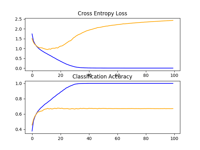
Line Plots of Learning Curves for VGG 1 Baseline on the CIFAR-10 Dataset
Baseline: 2 VGG Blocks
The define_model() function for two VGG blocks is listed below.
# define cnn model
def define_model():
        model = Sequential()
        model.add(Conv2D(32, (3, 3), activation='relu', kernel_initializer='he_uniform', padding='same', input_shape=(32, 32, 3)))
        model.add(Conv2D(32, (3, 3), activation='relu', kernel_initializer='he_uniform', padding='same'))
        model.add(MaxPooling2D((2, 2)))
        model.add(Conv2D(64, (3, 3), activation='relu', kernel_initializer='he_uniform', padding='same'))
        model.add(Conv2D(64, (3, 3), activation='relu', kernel_initializer='he_uniform', padding='same'))
        model.add(MaxPooling2D((2, 2)))
        model.add(Flatten())
        model.add(Dense(128, activation='relu', kernel_initializer='he_uniform'))
        model.add(Dense(10, activation='softmax'))
        # compile model
        opt = SGD(lr=0.001, momentum=0.9)
        model.compile(optimizer=opt, loss='categorical_crossentropy', metrics=['accuracy'])
        return model
Running the model in the test harness first prints the classification accuracy on the test dataset.
Your specific results may vary given the stochastic nature of the learning algorithm.
In this case, we can see that the model with two blocks performs better than the model with a single block: a good sign.
> 71.080
A figure showing learning curves is created and saved to file. In this case, we continue to see strong overfitting.
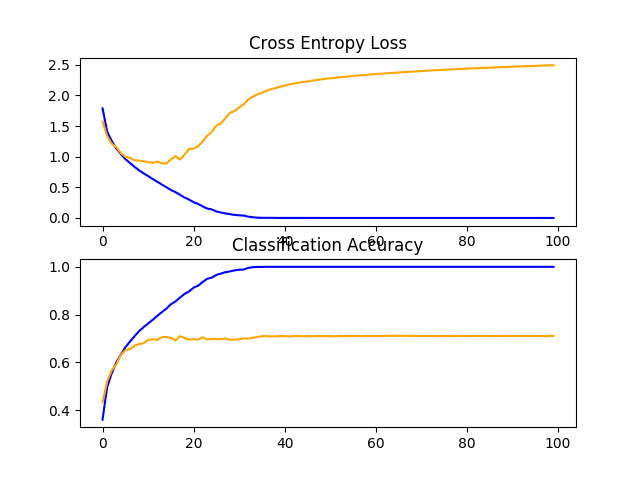
Line Plots of Learning Curves for VGG 2 Baseline on the CIFAR-10 Dataset
Baseline: 3 VGG Blocks
The define_model() function for three VGG blocks is listed below.
# define cnn model
def define_model():
        model = Sequential()
        model.add(Conv2D(32, (3, 3), activation='relu', kernel_initializer='he_uniform', padding='same', input_shape=(32, 32, 3)))
        model.add(Conv2D(32, (3, 3), activation='relu', kernel_initializer='he_uniform', padding='same'))
        model.add(MaxPooling2D((2, 2)))
        model.add(Conv2D(64, (3, 3), activation='relu', kernel_initializer='he_uniform', padding='same'))
        model.add(Conv2D(64, (3, 3), activation='relu', kernel_initializer='he_uniform', padding='same'))
        model.add(MaxPooling2D((2, 2)))
        model.add(Conv2D(128, (3, 3), activation='relu', kernel_initializer='he_uniform', padding='same'))
        model.add(Conv2D(128, (3, 3), activation='relu', kernel_initializer='he_uniform', padding='same'))
        model.add(MaxPooling2D((2, 2)))
        model.add(Flatten())
        model.add(Dense(128, activation='relu', kernel_initializer='he_uniform'))
        model.add(Dense(10, activation='softmax'))
        # compile model
        opt = SGD(lr=0.001, momentum=0.9)
        model.compile(optimizer=opt, loss='categorical_crossentropy', metrics=['accuracy'])
        return model
Running the model in the test harness first prints the classification accuracy on the test dataset.
Your specific results may vary given the stochastic nature of the learning algorithm.
In this case, yet another modest increase in performance is seen as the depth of the model was increased.
> 73.500
Reviewing the figures showing the learning curves, again we see dramatic overfitting within the first 20 training epochs.
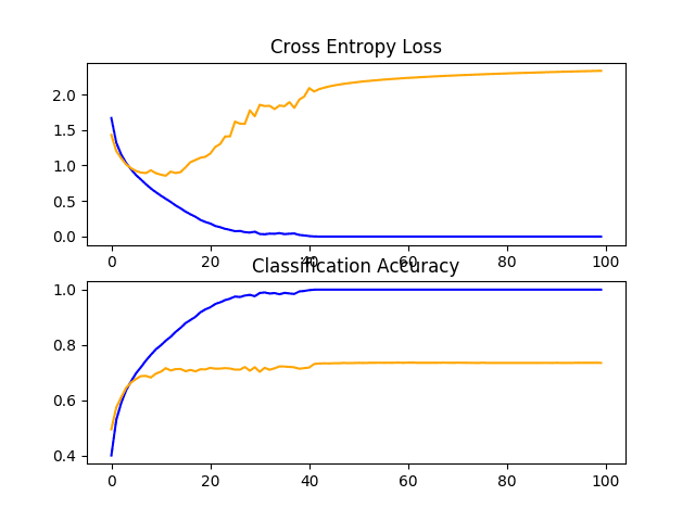
Line Plots of Learning Curves for VGG 3 Baseline on the CIFAR-10 Dataset
Discussion
We have explored three different models with a VGG-based architecture.
The results can be summarized below, although we must assume some variance in these results given the stochastic nature of the algorithm:
- VGG 1: 67.070%
- VGG 2: 71.080%
- VGG 3: 73.500%
In all cases, the model was able to learn the training dataset, showing an improvement on the training dataset that at least continued to 40 epochs, and perhaps more. This is a good sign, as it shows that the problem is learnable and that all three models have sufficient capacity to learn the problem.
The results of the model on the test dataset showed an improvement in classification accuracy with each increase in the depth of the model. It is possible that this trend would continue if models with four and five layers were evaluated, and this might make an interesting extension. Nevertheless, all three models showed the same pattern of dramatic overfitting at around 15-to-20 epochs.
These results suggest that the model with three VGG blocks is a good starting point or baseline model for our investigation.
The results also suggest that the model is in need of regularization to address the rapid overfitting of the test dataset. More generally, the results suggest that it may be useful to investigate techniques that slow down the convergence (rate of learning) of the model. This may include techniques such as data augmentation as well as learning rate schedules, changes to the batch size, and perhaps more.
In the next section, we will investigate some of these ideas for improving model performance.
How to Develop an Improved Model
Now that we have established a baseline model, the VGG architecture with three blocks, we can investigate modifications to the model and the training algorithm that seek to improve performance.
We will look at two main areas first to address the severe overfitting observed, namely regularization and data augmentation.
Regularization Techniques
There are many regularization techniques we could try, although the nature of the overfitting observed suggests that perhaps early stopping would not be appropriate and that techniques that slow down the rate of convergence might be useful.
We will look into the effect of both dropout and weight regularization or weight decay.
Dropout Regularization
Dropout is a simple technique that will randomly drop nodes out of the network. It has a regularizing effect as the remaining nodes must adapt to pick-up the slack of the removed nodes.
For more on dropout, see the post:
Dropout can be added to the model by adding new Dropout layers, where the amount of nodes removed is specified as a parameter. There are many patterns for adding Dropout to a model, in terms of where in the model to add the layers and how much dropout to use.
In this case, we will add Dropout layers after each max pooling layer and after the fully connected layer, and use a fixed dropout rate of 20% (e.g. retain 80% of the nodes).
The updated VGG 3 baseline model with dropout is listed below.
# define cnn model
def define_model():
        model = Sequential()
        model.add(Conv2D(32, (3, 3), activation='relu', kernel_initializer='he_uniform', padding='same', input_shape=(32, 32, 3)))
        model.add(Conv2D(32, (3, 3), activation='relu', kernel_initializer='he_uniform', padding='same'))
        model.add(MaxPooling2D((2, 2)))
        model.add(Dropout(0.2))
        model.add(Conv2D(64, (3, 3), activation='relu', kernel_initializer='he_uniform', padding='same'))
        model.add(Conv2D(64, (3, 3), activation='relu', kernel_initializer='he_uniform', padding='same'))
        model.add(MaxPooling2D((2, 2)))
        model.add(Dropout(0.2))
        model.add(Conv2D(128, (3, 3), activation='relu', kernel_initializer='he_uniform', padding='same'))
        model.add(Conv2D(128, (3, 3), activation='relu', kernel_initializer='he_uniform', padding='same'))
        model.add(MaxPooling2D((2, 2)))
        model.add(Dropout(0.2))
        model.add(Flatten())
        model.add(Dense(128, activation='relu', kernel_initializer='he_uniform'))
        model.add(Dropout(0.2))
        model.add(Dense(10, activation='softmax'))
        # compile model
        opt = SGD(lr=0.001, momentum=0.9)
        model.compile(optimizer=opt, loss='categorical_crossentropy', metrics=['accuracy'])
        return model
The full code listing is provided below for completeness.
# baseline model with dropout on the cifar10 dataset
import sys
from matplotlib import pyplot
from keras.datasets import cifar10
from keras.utils import to_categorical
from keras.models import Sequential
from keras.layers import Conv2D
from keras.layers import MaxPooling2D
from keras.layers import Dense
from keras.layers import Flatten
from keras.layers import Dropout
from keras.optimizers import SGD

# load train and test dataset
def load_dataset():
        # load dataset
        (trainX, trainY), (testX, testY) = cifar10.load_data()
        # one hot encode target values
        trainY = to_categorical(trainY)
        testY = to_categorical(testY)
        return trainX, trainY, testX, testY

# scale pixels
def prep_pixels(train, test):
        # convert from integers to floats
        train_norm = train.astype('float32')
        test_norm = test.astype('float32')
        # normalize to range 0-1
        train_norm = train_norm / 255.0
        test_norm = test_norm / 255.0
        # return normalized images
        return train_norm, test_norm

# define cnn model
def define_model():
        model = Sequential()
        model.add(Conv2D(32, (3, 3), activation='relu', kernel_initializer='he_uniform', padding='same', input_shape=(32, 32, 3)))
        model.add(Conv2D(32, (3, 3), activation='relu', kernel_initializer='he_uniform', padding='same'))
        model.add(MaxPooling2D((2, 2)))
        model.add(Dropout(0.2))
        model.add(Conv2D(64, (3, 3), activation='relu', kernel_initializer='he_uniform', padding='same'))
        model.add(Conv2D(64, (3, 3), activation='relu', kernel_initializer='he_uniform', padding='same'))
        model.add(MaxPooling2D((2, 2)))
        model.add(Dropout(0.2))
        model.add(Conv2D(128, (3, 3), activation='relu', kernel_initializer='he_uniform', padding='same'))
        model.add(Conv2D(128, (3, 3), activation='relu', kernel_initializer='he_uniform', padding='same'))
        model.add(MaxPooling2D((2, 2)))
        model.add(Dropout(0.2))
        model.add(Flatten())
        model.add(Dense(128, activation='relu', kernel_initializer='he_uniform'))
        model.add(Dropout(0.2))
        model.add(Dense(10, activation='softmax'))
        # compile model
        opt = SGD(lr=0.001, momentum=0.9)
        model.compile(optimizer=opt, loss='categorical_crossentropy', metrics=['accuracy'])
        return model

# plot diagnostic learning curves
def summarize_diagnostics(history):
        # plot loss
        pyplot.subplot(211)
        pyplot.title('Cross Entropy Loss')
        pyplot.plot(history.history['loss'], color='blue', label='train')
        pyplot.plot(history.history['val_loss'], color='orange', label='test')
        # plot accuracy
        pyplot.subplot(212)
        pyplot.title('Classification Accuracy')
        pyplot.plot(history.history['acc'], color='blue', label='train')
        pyplot.plot(history.history['val_acc'], color='orange', label='test')
        # save plot to file
        filename = sys.argv[0].split('/')[-1]
        pyplot.savefig(filename + '_plot.png')
        pyplot.close()

# run the test harness for evaluating a model
def run_test_harness():
        # load dataset
        trainX, trainY, testX, testY = load_dataset()
        # prepare pixel data
        trainX, testX = prep_pixels(trainX, testX)
        # define model
        model = define_model()
        # fit model
        history = model.fit(trainX, trainY, epochs=100, batch_size=64, validation_data=(testX, testY), verbose=0)
        # evaluate model
        _, acc = model.evaluate(testX, testY, verbose=0)
        print('> %.3f' % (acc * 100.0))
        # learning curves
        summarize_diagnostics(history)

# entry point, run the test harness
run_test_harness()
Running the model in the test harness prints the classification accuracy on the test dataset.
Your specific results may vary given the stochastic nature of the learning algorithm.
In this case, we can see a jump in classification accuracy by about 10% from about 73% without dropout to about 83% with dropout.
> 83.450
Reviewing the learning curve for the model, we can see that overfitting has been addressed. The model converges well for about 40 or 50 epochs, at which point there is no further improvement on the test dataset.
This is a great result. We could elaborate upon this model and add early stopping with a patience of about 10 epochs to save a well-performing model on the test set during training at around the point that no further improvements are observed.
We could also try exploring a learning rate schedule that drops the learning rate after improvements on the test set stall.
Dropout has performed well, and we do not know that the chosen rate of 20% is the best. We could explore other dropout rates, as well as differing positioning of the dropout layers in the model architecture.
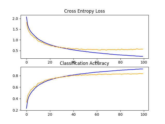
Line Plots of Learning Curves for Baseline Model With Dropout on the CIFAR-10 Dataset
Weight Decay
Weight regularization or weight decay involves updating the loss function to penalize the model in proportion to the size of the model weights.
This has a regularizing effect, as larger weights result in a more complex and less stable model, whereas smaller weights are often more stable and more general.
To learn more about weight regularization, see the post:
We can add weight regularization to the convolutional layers and the fully connected layers by defining the “kernel_regularizer” argument and specifying the type of regularization. In this case, we will use L2 weight regularization, the most common type used for neural networks and a sensible default weighting of 0.001.
The updated baseline model with weight decay is listed below.
# define cnn model
def define_model():
        model = Sequential()
        model.add(Conv2D(32, (3, 3), activation='relu', kernel_initializer='he_uniform', padding='same', kernel_regularizer=l2(0.001), input_shape=(32, 32, 3)))
        model.add(Conv2D(32, (3, 3), activation='relu', kernel_initializer='he_uniform', padding='same', kernel_regularizer=l2(0.001)))
        model.add(MaxPooling2D((2, 2)))
        model.add(Conv2D(64, (3, 3), activation='relu', kernel_initializer='he_uniform', padding='same', kernel_regularizer=l2(0.001)))
        model.add(Conv2D(64, (3, 3), activation='relu', kernel_initializer='he_uniform', padding='same', kernel_regularizer=l2(0.001)))
        model.add(MaxPooling2D((2, 2)))
        model.add(Conv2D(128, (3, 3), activation='relu', kernel_initializer='he_uniform', padding='same', kernel_regularizer=l2(0.001)))
        model.add(Conv2D(128, (3, 3), activation='relu', kernel_initializer='he_uniform', padding='same', kernel_regularizer=l2(0.001)))
        model.add(MaxPooling2D((2, 2)))
        model.add(Flatten())
        model.add(Dense(128, activation='relu', kernel_initializer='he_uniform', kernel_regularizer=l2(0.001)))
        model.add(Dense(10, activation='softmax'))
        # compile model
        opt = SGD(lr=0.001, momentum=0.9)
        model.compile(optimizer=opt, loss='categorical_crossentropy', metrics=['accuracy'])
        return model
The full code listing is provided below for completeness.
# baseline model with weight decay on the cifar10 dataset
import sys
from matplotlib import pyplot
from keras.datasets import cifar10
from keras.utils import to_categorical
from keras.models import Sequential
from keras.layers import Conv2D
from keras.layers import MaxPooling2D
from keras.layers import Dense
from keras.layers import Flatten
from keras.optimizers import SGD
from keras.regularizers import l2

# load train and test dataset
def load_dataset():
        # load dataset
        (trainX, trainY), (testX, testY) = cifar10.load_data()
        # one hot encode target values
        trainY = to_categorical(trainY)
        testY = to_categorical(testY)
        return trainX, trainY, testX, testY

# scale pixels
def prep_pixels(train, test):
        # convert from integers to floats
        train_norm = train.astype('float32')
        test_norm = test.astype('float32')
        # normalize to range 0-1
        train_norm = train_norm / 255.0
        test_norm = test_norm / 255.0
        # return normalized images
        return train_norm, test_norm

# define cnn model
def define_model():
        model = Sequential()
        model.add(Conv2D(32, (3, 3), activation='relu', kernel_initializer='he_uniform', padding='same', kernel_regularizer=l2(0.001), input_shape=(32, 32, 3)))
        model.add(Conv2D(32, (3, 3), activation='relu', kernel_initializer='he_uniform', padding='same', kernel_regularizer=l2(0.001)))
        model.add(MaxPooling2D((2, 2)))
        model.add(Conv2D(64, (3, 3), activation='relu', kernel_initializer='he_uniform', padding='same', kernel_regularizer=l2(0.001)))
        model.add(Conv2D(64, (3, 3), activation='relu', kernel_initializer='he_uniform', padding='same', kernel_regularizer=l2(0.001)))
        model.add(MaxPooling2D((2, 2)))
        model.add(Conv2D(128, (3, 3), activation='relu', kernel_initializer='he_uniform', padding='same', kernel_regularizer=l2(0.001)))
        model.add(Conv2D(128, (3, 3), activation='relu', kernel_initializer='he_uniform', padding='same', kernel_regularizer=l2(0.001)))
        model.add(MaxPooling2D((2, 2)))
        model.add(Flatten())
        model.add(Dense(128, activation='relu', kernel_initializer='he_uniform', kernel_regularizer=l2(0.001)))
        model.add(Dense(10, activation='softmax'))
        # compile model
        opt = SGD(lr=0.001, momentum=0.9)
        model.compile(optimizer=opt, loss='categorical_crossentropy', metrics=['accuracy'])
        return model

# plot diagnostic learning curves
def summarize_diagnostics(history):
        # plot loss
        pyplot.subplot(211)
        pyplot.title('Cross Entropy Loss')
        pyplot.plot(history.history['loss'], color='blue', label='train')
        pyplot.plot(history.history['val_loss'], color='orange', label='test')
        # plot accuracy
        pyplot.subplot(212)
        pyplot.title('Classification Accuracy')
        pyplot.plot(history.history['acc'], color='blue', label='train')
        pyplot.plot(history.history['val_acc'], color='orange', label='test')
        # save plot to file
        filename = sys.argv[0].split('/')[-1]
        pyplot.savefig(filename + '_plot.png')
        pyplot.close()

# run the test harness for evaluating a model
def run_test_harness():
        # load dataset
        trainX, trainY, testX, testY = load_dataset()
        # prepare pixel data
        trainX, testX = prep_pixels(trainX, testX)
        # define model
        model = define_model()
        # fit model
        history = model.fit(trainX, trainY, epochs=100, batch_size=64, validation_data=(testX, testY), verbose=0)
        # evaluate model
        _, acc = model.evaluate(testX, testY, verbose=0)
        print('> %.3f' % (acc * 100.0))
        # learning curves
        summarize_diagnostics(history)

# entry point, run the test harness
run_test_harness()
Running the model in the test harness prints the classification accuracy of the test dataset.
Your specific results may vary given the stochastic nature of the learning algorithm.
In this case, we see no improvement in the model performance on the test set; in fact, we see a small drop in performance from about 73% to about 72% classification accuracy.
> 72.550
Reviewing the learning curves, we do see a small reduction in the overfitting, but the impact is not as effective as dropout.
We might be able to improve the effect of weight decay by perhaps using a larger weighting, such as 0.01 or even 0.1.
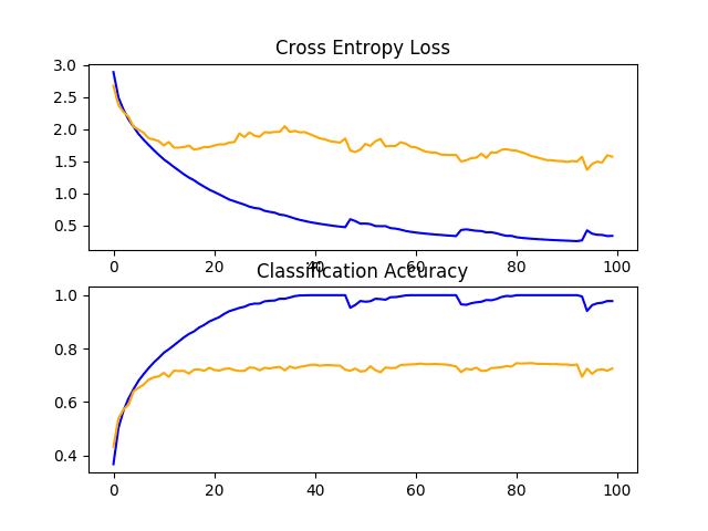
Line Plots of Learning Curves for Baseline Model With Weight Decay on the CIFAR-10 Dataset
Data Augmentation
Data augmentation involves making copies of the examples in the training dataset with small random modifications.
This has a regularizing effect as it both expands the training dataset and allows the model to learn the same general features, although in a more generalized manner.
There are many types of data augmentation that could be applied. Given that the dataset is comprised of small photos of objects, we do not want to use augmentation that distorts the images too much, so that useful features in the images can be preserved and used.
The types of random augmentations that could be useful include a horizontal flip, minor shifts of the image, and perhaps small zooming or cropping of the image.
We will investigate the effect of simple augmentation on the baseline image, specifically horizontal flips and 10% shifts in the height and width of the image.
This can be implemented in Keras using the ImageDataGenerator class; for example:
# create data generator
datagen = ImageDataGenerator(width_shift_range=0.1, height_shift_range=0.1, horizontal_flip=True)
# prepare iterator
it_train = datagen.flow(trainX, trainY, batch_size=64)
This can be used during training by passing the iterator to the model.fit_generator() function and defining the number of batches in a single epoch.
# fit model
steps = int(trainX.shape[0] / 64)
history = model.fit_generator(it_train, steps_per_epoch=steps, epochs=100, validation_data=(testX, testY), verbose=0)
No changes to the model are required.
The updated version of the run_test_harness() function to support data augmentation is listed below.
# run the test harness for evaluating a model
def run_test_harness():
        # load dataset
        trainX, trainY, testX, testY = load_dataset()
        # prepare pixel data
        trainX, testX = prep_pixels(trainX, testX)
        # define model
        model = define_model()
        # create data generator
        datagen = ImageDataGenerator(width_shift_range=0.1, height_shift_range=0.1, horizontal_flip=True)
        # prepare iterator
        it_train = datagen.flow(trainX, trainY, batch_size=64)
        # fit model
        steps = int(trainX.shape[0] / 64)
        history = model.fit_generator(it_train, steps_per_epoch=steps, epochs=100, validation_data=(testX, testY), verbose=0)
        # evaluate model
        _, acc = model.evaluate(testX, testY, verbose=0)
        print('> %.3f' % (acc * 100.0))
        # learning curves
        summarize_diagnostics(history)
The full code listing is provided below for completeness.
# baseline model with data augmentation on the cifar10 dataset
import sys
from matplotlib import pyplot
from keras.datasets import cifar10
from keras.utils import to_categorical
from keras.models import Sequential
from keras.layers import Conv2D
from keras.layers import MaxPooling2D
from keras.layers import Dense
from keras.layers import Flatten
from keras.optimizers import SGD
from keras.preprocessing.image import ImageDataGenerator

# load train and test dataset
def load_dataset():
        # load dataset
        (trainX, trainY), (testX, testY) = cifar10.load_data()
        # one hot encode target values
        trainY = to_categorical(trainY)
        testY = to_categorical(testY)
        return trainX, trainY, testX, testY

# scale pixels
def prep_pixels(train, test):
        # convert from integers to floats
        train_norm = train.astype('float32')
        test_norm = test.astype('float32')
        # normalize to range 0-1
        train_norm = train_norm / 255.0
        test_norm = test_norm / 255.0
        # return normalized images
        return train_norm, test_norm

# define cnn model
def define_model():
        model = Sequential()
        model.add(Conv2D(32, (3, 3), activation='relu', kernel_initializer='he_uniform', padding='same', input_shape=(32, 32, 3)))
        model.add(Conv2D(32, (3, 3), activation='relu', kernel_initializer='he_uniform', padding='same'))
        model.add(MaxPooling2D((2, 2)))
        model.add(Conv2D(64, (3, 3), activation='relu', kernel_initializer='he_uniform', padding='same'))
        model.add(Conv2D(64, (3, 3), activation='relu', kernel_initializer='he_uniform', padding='same'))
        model.add(MaxPooling2D((2, 2)))
        model.add(Conv2D(128, (3, 3), activation='relu', kernel_initializer='he_uniform', padding='same'))
        model.add(Conv2D(128, (3, 3), activation='relu', kernel_initializer='he_uniform', padding='same'))
        model.add(MaxPooling2D((2, 2)))
        model.add(Flatten())
        model.add(Dense(128, activation='relu', kernel_initializer='he_uniform'))
        model.add(Dense(10, activation='softmax'))
        # compile model
        opt = SGD(lr=0.001, momentum=0.9)
        model.compile(optimizer=opt, loss='categorical_crossentropy', metrics=['accuracy'])
        return model

# plot diagnostic learning curves
def summarize_diagnostics(history):
        # plot loss
        pyplot.subplot(211)
        pyplot.title('Cross Entropy Loss')
        pyplot.plot(history.history['loss'], color='blue', label='train')
        pyplot.plot(history.history['val_loss'], color='orange', label='test')
        # plot accuracy
        pyplot.subplot(212)
        pyplot.title('Classification Accuracy')
        pyplot.plot(history.history['acc'], color='blue', label='train')
        pyplot.plot(history.history['val_acc'], color='orange', label='test')
        # save plot to file
        filename = sys.argv[0].split('/')[-1]
        pyplot.savefig(filename + '_plot.png')
        pyplot.close()

# run the test harness for evaluating a model
def run_test_harness():
        # load dataset
        trainX, trainY, testX, testY = load_dataset()
        # prepare pixel data
        trainX, testX = prep_pixels(trainX, testX)
        # define model
        model = define_model()
        # create data generator
        datagen = ImageDataGenerator(width_shift_range=0.1, height_shift_range=0.1, horizontal_flip=True)
        # prepare iterator
        it_train = datagen.flow(trainX, trainY, batch_size=64)
        # fit model
        steps = int(trainX.shape[0] / 64)
        history = model.fit_generator(it_train, steps_per_epoch=steps, epochs=100, validation_data=(testX, testY), verbose=0)
        # evaluate model
        _, acc = model.evaluate(testX, testY, verbose=0)
        print('> %.3f' % (acc * 100.0))
        # learning curves
        summarize_diagnostics(history)

# entry point, run the test harness
run_test_harness()
Running the model in the test harness prints the classification accuracy on the test dataset.
Your specific results may vary given the stochastic nature of the learning algorithm.
In this case, we see another large improvement in model performance, much like we saw with dropout. In this case, an improvement of about 11% from about 73% for the baseline model to about 84%.
> 84.470
Reviewing the learning curves, we see a similar improvement in model performances as we do with dropout, although the plot of loss suggests that model performance on the test set may have stalled slightly sooner than it did with dropout.
The results suggest that perhaps a configuration that used both dropout and data augmentation might be effective.
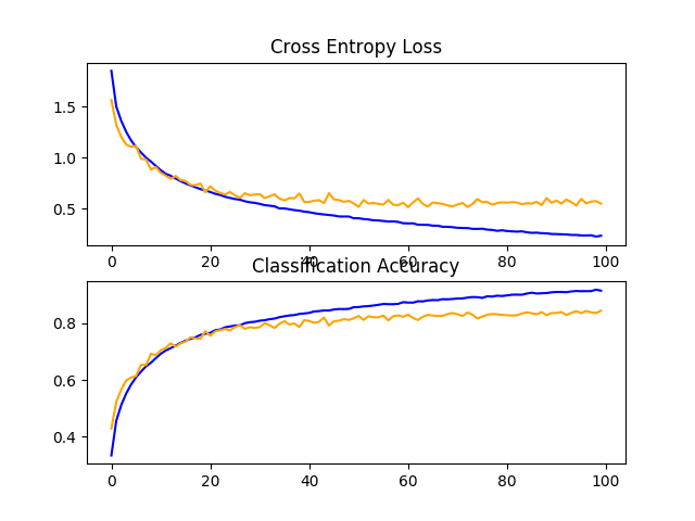
Line Plots of Learning Curves for Baseline Model With Data Augmentation on the CIFAR-10 Dataset
Discussion
In this section, we explored three approaches designed to slow down the convergence of the model.
A summary of the results is provided below:
- Baseline + Dropout: 83.450%
- Baseline + Weight Decay: 72.550%
- Baseline + Data Augmentation: 84.470%
The results suggest that both dropout and data augmentation are having the desired effect, and weight decay, at least for the chosen configuration, did not.
Now that the model is learning well, we can look for both improvements on what is working, as well as combinations on what is working.
How to Develop Further Improvements
In the previous section, we discovered that dropout and data augmentation, when added to the baseline model, result in a model that learns the problem well.
We will now investigate refinements of these techniques to see if we can further improve the model’s performance. Specifically, we will look at a variation of dropout regularization and combining dropout with data augmentation.
Learning has slowed down, so we will investigate increasing the number of training epochs to give the model enough space, if needed, to expose the learning dynamics in the learning curves.
Variation of Dropout Regularization
Dropout is working very well, so it may be worth investigating variations of how dropout is applied to the model.
One variation that might be interesting is to increase the amount of dropout from 20% to 25% or 30%. Another variation that might be interesting is using a pattern of increasing dropout from 20% for the first block, 30% for the second block, and so on to 50% at the fully connected layer in the classifier part of the model.
This type of increasing dropout with the depth of the model is a common pattern. It is effective as it forces layers deep in the model to regularize more than layers closer to the input.
The baseline model with dropout updated to use a pattern of increasing dropout percentage with model depth is defined below.
# define cnn model
def define_model():
        model = Sequential()
        model.add(Conv2D(32, (3, 3), activation='relu', kernel_initializer='he_uniform', padding='same', input_shape=(32, 32, 3)))
        model.add(Conv2D(32, (3, 3), activation='relu', kernel_initializer='he_uniform', padding='same'))
        model.add(MaxPooling2D((2, 2)))
        model.add(Dropout(0.2))
        model.add(Conv2D(64, (3, 3), activation='relu', kernel_initializer='he_uniform', padding='same'))
        model.add(Conv2D(64, (3, 3), activation='relu', kernel_initializer='he_uniform', padding='same'))
        model.add(MaxPooling2D((2, 2)))
        model.add(Dropout(0.3))
        model.add(Conv2D(128, (3, 3), activation='relu', kernel_initializer='he_uniform', padding='same'))
        model.add(Conv2D(128, (3, 3), activation='relu', kernel_initializer='he_uniform', padding='same'))
        model.add(MaxPooling2D((2, 2)))
        model.add(Dropout(0.4))
        model.add(Flatten())
        model.add(Dense(128, activation='relu', kernel_initializer='he_uniform'))
        model.add(Dropout(0.5))
        model.add(Dense(10, activation='softmax'))
        # compile model
        opt = SGD(lr=0.001, momentum=0.9)
        model.compile(optimizer=opt, loss='categorical_crossentropy', metrics=['accuracy'])
        return model
The full code listing with this change is provided below for completeness.
# baseline model with increasing dropout on the cifar10 dataset
import sys
from matplotlib import pyplot
from keras.datasets import cifar10
from keras.utils import to_categorical
from keras.models import Sequential
from keras.layers import Conv2D
from keras.layers import MaxPooling2D
from keras.layers import Dense
from keras.layers import Flatten
from keras.layers import Dropout
from keras.optimizers import SGD

# load train and test dataset
def load_dataset():
        # load dataset
        (trainX, trainY), (testX, testY) = cifar10.load_data()
        # one hot encode target values
        trainY = to_categorical(trainY)
        testY = to_categorical(testY)
        return trainX, trainY, testX, testY

# scale pixels
def prep_pixels(train, test):
        # convert from integers to floats
        train_norm = train.astype('float32')
        test_norm = test.astype('float32')
        # normalize to range 0-1
        train_norm = train_norm / 255.0
        test_norm = test_norm / 255.0
        # return normalized images
        return train_norm, test_norm

# define cnn model
def define_model():
        model = Sequential()
        model.add(Conv2D(32, (3, 3), activation='relu', kernel_initializer='he_uniform', padding='same', input_shape=(32, 32, 3)))
        model.add(Conv2D(32, (3, 3), activation='relu', kernel_initializer='he_uniform', padding='same'))
        model.add(MaxPooling2D((2, 2)))
        model.add(Dropout(0.2))
        model.add(Conv2D(64, (3, 3), activation='relu', kernel_initializer='he_uniform', padding='same'))
        model.add(Conv2D(64, (3, 3), activation='relu', kernel_initializer='he_uniform', padding='same'))
        model.add(MaxPooling2D((2, 2)))
        model.add(Dropout(0.3))
        model.add(Conv2D(128, (3, 3), activation='relu', kernel_initializer='he_uniform', padding='same'))
        model.add(Conv2D(128, (3, 3), activation='relu', kernel_initializer='he_uniform', padding='same'))
        model.add(MaxPooling2D((2, 2)))
        model.add(Dropout(0.4))
        model.add(Flatten())
        model.add(Dense(128, activation='relu', kernel_initializer='he_uniform'))
        model.add(Dropout(0.5))
        model.add(Dense(10, activation='softmax'))
        # compile model
        opt = SGD(lr=0.001, momentum=0.9)
        model.compile(optimizer=opt, loss='categorical_crossentropy', metrics=['accuracy'])
        return model

# plot diagnostic learning curves
def summarize_diagnostics(history):
        # plot loss
        pyplot.subplot(211)
        pyplot.title('Cross Entropy Loss')
        pyplot.plot(history.history['loss'], color='blue', label='train')
        pyplot.plot(history.history['val_loss'], color='orange', label='test')
        # plot accuracy
        pyplot.subplot(212)
        pyplot.title('Classification Accuracy')
        pyplot.plot(history.history['acc'], color='blue', label='train')
        pyplot.plot(history.history['val_acc'], color='orange', label='test')
        # save plot to file
        filename = sys.argv[0].split('/')[-1]
        pyplot.savefig(filename + '_plot.png')
        pyplot.close()

# run the test harness for evaluating a model
def run_test_harness():
        # load dataset
        trainX, trainY, testX, testY = load_dataset()
        # prepare pixel data
        trainX, testX = prep_pixels(trainX, testX)
        # define model
        model = define_model()
        # fit model
        history = model.fit(trainX, trainY, epochs=200, batch_size=64, validation_data=(testX, testY), verbose=0)
        # evaluate model
        _, acc = model.evaluate(testX, testY, verbose=0)
        print('> %.3f' % (acc * 100.0))
        # learning curves
        summarize_diagnostics(history)

# entry point, run the test harness
run_test_harness()
Running the model in the test harness prints the classification accuracy on the test dataset.
Your specific results may vary given the stochastic nature of the learning algorithm.
In this case, we can see a modest lift in performance from fixed dropout at about 83% to increasing dropout at about 84%.
> 84.690
Reviewing the learning curves, we can see that the model converges well, with performance on the test dataset perhaps stalling at around 110 to 125 epochs. Compared to the learning curves for fixed dropout, we can see that again the rate of learning has been further slowed, allowing further refinement of the model without overfitting.
This is a fruitful area for investigation on this model, and perhaps more dropout layers and/or more aggressive dropout may result in further improvements.
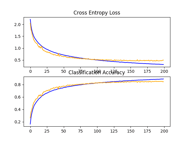
Line Plots of Learning Curves for Baseline Model With Increasing Dropout on the CIFAR-10 Dataset
Dropout and Data Augmentation
In the previous section, we discovered that both dropout and data augmentation resulted in a significant improvement in model performance.
In this section, we can experiment with combining both of these changes to the model to see if a further improvement can be achieved. Specifically, whether using both regularization techniques together results in better performance than either technique used alone.
The full code listing of a model with fixed dropout and data augmentation is provided below for completeness.
# baseline model with dropout and data augmentation on the cifar10 dataset
import sys
from matplotlib import pyplot
from keras.datasets import cifar10
from keras.utils import to_categorical
from keras.models import Sequential
from keras.layers import Conv2D
from keras.layers import MaxPooling2D
from keras.layers import Dense
from keras.layers import Flatten
from keras.optimizers import SGD
from keras.preprocessing.image import ImageDataGenerator
from keras.layers import Dropout

# load train and test dataset
def load_dataset():
        # load dataset
        (trainX, trainY), (testX, testY) = cifar10.load_data()
        # one hot encode target values
        trainY = to_categorical(trainY)
        testY = to_categorical(testY)
        return trainX, trainY, testX, testY

# scale pixels
def prep_pixels(train, test):
        # convert from integers to floats
        train_norm = train.astype('float32')
        test_norm = test.astype('float32')
        # normalize to range 0-1
        train_norm = train_norm / 255.0
        test_norm = test_norm / 255.0
        # return normalized images
        return train_norm, test_norm

# define cnn model
def define_model():
        model = Sequential()
        model.add(Conv2D(32, (3, 3), activation='relu', kernel_initializer='he_uniform', padding='same', input_shape=(32, 32, 3)))
        model.add(Conv2D(32, (3, 3), activation='relu', kernel_initializer='he_uniform', padding='same'))
        model.add(MaxPooling2D((2, 2)))
        model.add(Dropout(0.2))
        model.add(Conv2D(64, (3, 3), activation='relu', kernel_initializer='he_uniform', padding='same'))
        model.add(Conv2D(64, (3, 3), activation='relu', kernel_initializer='he_uniform', padding='same'))
        model.add(MaxPooling2D((2, 2)))
        model.add(Dropout(0.2))
        model.add(Conv2D(128, (3, 3), activation='relu', kernel_initializer='he_uniform', padding='same'))
        model.add(Conv2D(128, (3, 3), activation='relu', kernel_initializer='he_uniform', padding='same'))
        model.add(MaxPooling2D((2, 2)))
        model.add(Dropout(0.2))
        model.add(Flatten())
        model.add(Dense(128, activation='relu', kernel_initializer='he_uniform'))
        model.add(Dropout(0.2))
        model.add(Dense(10, activation='softmax'))
        # compile model
        opt = SGD(lr=0.001, momentum=0.9)
        model.compile(optimizer=opt, loss='categorical_crossentropy', metrics=['accuracy'])
        return model

# plot diagnostic learning curves
def summarize_diagnostics(history):
        # plot loss
        pyplot.subplot(211)
        pyplot.title('Cross Entropy Loss')
        pyplot.plot(history.history['loss'], color='blue', label='train')
        pyplot.plot(history.history['val_loss'], color='orange', label='test')
        # plot accuracy
        pyplot.subplot(212)
        pyplot.title('Classification Accuracy')
        pyplot.plot(history.history['acc'], color='blue', label='train')
        pyplot.plot(history.history['val_acc'], color='orange', label='test')
        # save plot to file
        filename = sys.argv[0].split('/')[-1]
        pyplot.savefig(filename + '_plot.png')
        pyplot.close()

# run the test harness for evaluating a model
def run_test_harness():
        # load dataset
        trainX, trainY, testX, testY = load_dataset()
        # prepare pixel data
        trainX, testX = prep_pixels(trainX, testX)
        # define model
        model = define_model()
        # create data generator
        datagen = ImageDataGenerator(width_shift_range=0.1, height_shift_range=0.1, horizontal_flip=True)
        # prepare iterator
        it_train = datagen.flow(trainX, trainY, batch_size=64)
        # fit model
        steps = int(trainX.shape[0] / 64)
        history = model.fit_generator(it_train, steps_per_epoch=steps, epochs=200, validation_data=(testX, testY), verbose=0)
        # evaluate model
        _, acc = model.evaluate(testX, testY, verbose=0)
        print('> %.3f' % (acc * 100.0))
        # learning curves
        summarize_diagnostics(history)

# entry point, run the test harness
run_test_harness()
Running the model in the test harness prints the classification accuracy on the test dataset.
Your specific results may vary given the stochastic nature of the learning algorithm.
In this case, we can see that as we would have hoped, using both regularization techniques together has resulted in a further lift in model performance on the test set. In this case, combining fixed dropout with about 83% and data augmentation with about 84% has resulted in an improvement to about 85% classification accuracy.
> 85.880
Reviewing the learning curves, we can see that the convergence behavior of the model is also better than either fixed dropout and data augmentation alone. Learning has been slowed without overfitting, allowing continued improvement.
The plot also suggests that learning may not have stalled and may have continued to improve if allowed to continue, but perhaps very modestly.
Results might be further improved if a pattern of increasing dropout was used instead of a fixed dropout rate throughout the depth of the model.
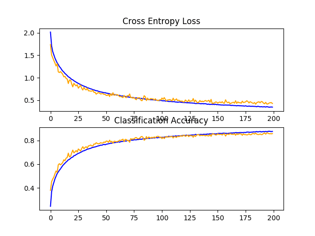
Line Plots of Learning Curves for Baseline Model With Dropout and Data Augmentation on the CIFAR-10 Dataset
Dropout and Data Augmentation and Batch Normalization
We can expand upon the previous example in a few ways.
First, we can increase the number of training epochs from 200 to 400, to give the model more of an opportunity to improve.
Next, we can add batch normalization in an effort to stabilize the learning and perhaps accelerate the learning process. To offset this acceleration, we can increase the regularization by changing the dropout from a fixed pattern to an increasing pattern.
The updated model definition is listed below.
# define cnn model
def define_model():
        model = Sequential()
        model.add(Conv2D(32, (3, 3), activation='relu', kernel_initializer='he_uniform', padding='same', input_shape=(32, 32, 3)))
        model.add(BatchNormalization())
        model.add(Conv2D(32, (3, 3), activation='relu', kernel_initializer='he_uniform', padding='same'))
        model.add(BatchNormalization())
        model.add(MaxPooling2D((2, 2)))
        model.add(Dropout(0.2))
        model.add(Conv2D(64, (3, 3), activation='relu', kernel_initializer='he_uniform', padding='same'))
        model.add(BatchNormalization())
        model.add(Conv2D(64, (3, 3), activation='relu', kernel_initializer='he_uniform', padding='same'))
        model.add(BatchNormalization())
        model.add(MaxPooling2D((2, 2)))
        model.add(Dropout(0.3))
        model.add(Conv2D(128, (3, 3), activation='relu', kernel_initializer='he_uniform', padding='same'))
        model.add(BatchNormalization())
        model.add(Conv2D(128, (3, 3), activation='relu', kernel_initializer='he_uniform', padding='same'))
        model.add(BatchNormalization())
        model.add(MaxPooling2D((2, 2)))
        model.add(Dropout(0.4))
        model.add(Flatten())
        model.add(Dense(128, activation='relu', kernel_initializer='he_uniform'))
        model.add(BatchNormalization())
        model.add(Dropout(0.5))
        model.add(Dense(10, activation='softmax'))
        # compile model
        opt = SGD(lr=0.001, momentum=0.9)
        model.compile(optimizer=opt, loss='categorical_crossentropy', metrics=['accuracy'])
        return model
The full code listing of a model with increasing dropout, data augmentation, batch normalization, and 400 training epochs is provided below for completeness.
# baseline model with dropout and data augmentation on the cifar10 dataset
import sys
from matplotlib import pyplot
from keras.datasets import cifar10
from keras.utils import to_categorical
from keras.models import Sequential
from keras.layers import Conv2D
from keras.layers import MaxPooling2D
from keras.layers import Dense
from keras.layers import Flatten
from keras.optimizers import SGD
from keras.preprocessing.image import ImageDataGenerator
from keras.layers import Dropout
from keras.layers import BatchNormalization

# load train and test dataset
def load_dataset():
        # load dataset
        (trainX, trainY), (testX, testY) = cifar10.load_data()
        # one hot encode target values
        trainY = to_categorical(trainY)
        testY = to_categorical(testY)
        return trainX, trainY, testX, testY

# scale pixels
def prep_pixels(train, test):
        # convert from integers to floats
        train_norm = train.astype('float32')
        test_norm = test.astype('float32')
        # normalize to range 0-1
        train_norm = train_norm / 255.0
        test_norm = test_norm / 255.0
        # return normalized images
        return train_norm, test_norm

# define cnn model
def define_model():
        model = Sequential()
        model.add(Conv2D(32, (3, 3), activation='relu', kernel_initializer='he_uniform', padding='same', input_shape=(32, 32, 3)))
        model.add(BatchNormalization())
        model.add(Conv2D(32, (3, 3), activation='relu', kernel_initializer='he_uniform', padding='same'))
        model.add(BatchNormalization())
        model.add(MaxPooling2D((2, 2)))
        model.add(Dropout(0.2))
        model.add(Conv2D(64, (3, 3), activation='relu', kernel_initializer='he_uniform', padding='same'))
        model.add(BatchNormalization())
        model.add(Conv2D(64, (3, 3), activation='relu', kernel_initializer='he_uniform', padding='same'))
        model.add(BatchNormalization())
        model.add(MaxPooling2D((2, 2)))
        model.add(Dropout(0.3))
        model.add(Conv2D(128, (3, 3), activation='relu', kernel_initializer='he_uniform', padding='same'))
        model.add(BatchNormalization())
        model.add(Conv2D(128, (3, 3), activation='relu', kernel_initializer='he_uniform', padding='same'))
        model.add(BatchNormalization())
        model.add(MaxPooling2D((2, 2)))
        model.add(Dropout(0.4))
        model.add(Flatten())
        model.add(Dense(128, activation='relu', kernel_initializer='he_uniform'))
        model.add(BatchNormalization())
        model.add(Dropout(0.5))
        model.add(Dense(10, activation='softmax'))
        # compile model
        opt = SGD(lr=0.001, momentum=0.9)
        model.compile(optimizer=opt, loss='categorical_crossentropy', metrics=['accuracy'])
        return model

# plot diagnostic learning curves
def summarize_diagnostics(history):
        # plot loss
        pyplot.subplot(211)
        pyplot.title('Cross Entropy Loss')
        pyplot.plot(history.history['loss'], color='blue', label='train')
        pyplot.plot(history.history['val_loss'], color='orange', label='test')
        # plot accuracy
        pyplot.subplot(212)
        pyplot.title('Classification Accuracy')
        pyplot.plot(history.history['acc'], color='blue', label='train')
        pyplot.plot(history.history['val_acc'], color='orange', label='test')
        # save plot to file
        filename = sys.argv[0].split('/')[-1]
        pyplot.savefig(filename + '_plot.png')
        pyplot.close()

# run the test harness for evaluating a model
def run_test_harness():
        # load dataset
        trainX, trainY, testX, testY = load_dataset()
        # prepare pixel data
        trainX, testX = prep_pixels(trainX, testX)
        # define model
        model = define_model()
        # create data generator
        datagen = ImageDataGenerator(width_shift_range=0.1, height_shift_range=0.1, horizontal_flip=True)
        # prepare iterator
        it_train = datagen.flow(trainX, trainY, batch_size=64)
        # fit model
        steps = int(trainX.shape[0] / 64)
        history = model.fit_generator(it_train, steps_per_epoch=steps, epochs=400, validation_data=(testX, testY), verbose=0)
        # evaluate model
        _, acc = model.evaluate(testX, testY, verbose=0)
        print('> %.3f' % (acc * 100.0))
        # learning curves
        summarize_diagnostics(history)

# entry point, run the test harness
run_test_harness()
Running the model in the test harness prints the classification accuracy on the test dataset.
Your specific results may vary given the stochastic nature of the learning algorithm.
In this case, we can see that we achieved a further lift in model performance to about 88% accuracy, improving upon both dropout and data augmentation alone at about 84% and upon the increasing dropout alone at about 85%.
> 88.620
Reviewing the learning curves, we can see the training of the model shows continued improvement for nearly the duration of 400 epochs. We can see perhaps a slight drop-off on the test dataset at around 300 epochs, but the improvement trend does continue.
The model may benefit from further training epochs.
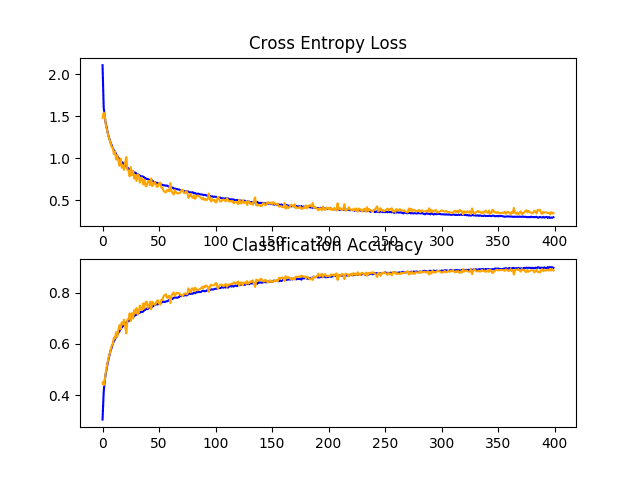
Line Plots of Learning Curves for Baseline Model With Increasing Dropout, Data Augmentation, and Batch Normalization on the CIFAR-10 Dataset
Discussion
In this section, we explored two approaches designed to expand upon changes to the model that we know already result in an improvement
A summary of the results is provided below:
- Baseline + Increasing Dropout: 84.690%
- Baseline + Dropout + Data Augmentation: 85.880%
- Baseline + Increasing Dropout + Data Augmentation + Batch Normalization: 88.620%
The model is now learning well and we have good control over the rate of learning without overfitting.
We might be able to achieve further improvements with additional regularization. This could be achieved with more aggressive dropout in later layers. It is possible that further addition of weight decay may improve the model.
So far, we have not tuned the hyperparameters of the learning algorithm, such as the learning rate, which is perhaps the most important hyperparameter. We may expect further improvements with adaptive changes to the learning rate, such as use of an adaptive learning rate technique such as Adam. These types of changes may help to refine the model once converged.
How to Finalize the Model and Make Predictions
The process of model improvement may continue for as long as we have ideas and the time and resources to test them out.
At some point, a final model configuration must be chosen and adopted. In this case, we will keep things simple and use the baseline model (VGG with 3 blocks) as the final model.
First, we will finalize our model by fitting a model on the entire training dataset and saving the model to file for later use. We will then load the model and evaluate its performance on the hold out test dataset, to get an idea of how well the chosen model actually performs in practice. Finally, we will use the saved model to make a prediction on a single image.
Save Final Model
A final model is typically fit on all available data, such as the combination of all train and test dataset.
In this tutorial, we will demonstrate the final model fit only on the just training dataset to keep the example simple.
The first step is to fit the final model on the entire training dataset.
# fit model
model.fit(trainX, trainY, epochs=100, batch_size=64, verbose=0)
Once fit, we can save the final model to an H5 file by calling the save() function on the model and pass in the chosen filename.
# save model
model.save('final_model.h5')
Note: saving and loading a Keras model requires that the h5py library is installed on your workstation.
The complete example of fitting the final model on the training dataset and saving it to file is listed below.
# save the final model to file
from keras.datasets import cifar10
from keras.utils import to_categorical
from keras.models import Sequential
from keras.layers import Conv2D
from keras.layers import MaxPooling2D
from keras.layers import Dense
from keras.layers import Flatten
from keras.optimizers import SGD

# load train and test dataset
def load_dataset():
        # load dataset
        (trainX, trainY), (testX, testY) = cifar10.load_data()
        # one hot encode target values
        trainY = to_categorical(trainY)
        testY = to_categorical(testY)
        return trainX, trainY, testX, testY

# scale pixels
def prep_pixels(train, test):
        # convert from integers to floats
        train_norm = train.astype('float32')
        test_norm = test.astype('float32')
        # normalize to range 0-1
        train_norm = train_norm / 255.0
        test_norm = test_norm / 255.0
        # return normalized images
        return train_norm, test_norm

# define cnn model
def define_model():
        model = Sequential()
        model.add(Conv2D(32, (3, 3), activation='relu', kernel_initializer='he_uniform', padding='same', input_shape=(32, 32, 3)))
        model.add(Conv2D(32, (3, 3), activation='relu', kernel_initializer='he_uniform', padding='same'))
        model.add(MaxPooling2D((2, 2)))
        model.add(Conv2D(64, (3, 3), activation='relu', kernel_initializer='he_uniform', padding='same'))
        model.add(Conv2D(64, (3, 3), activation='relu', kernel_initializer='he_uniform', padding='same'))
        model.add(MaxPooling2D((2, 2)))
        model.add(Conv2D(128, (3, 3), activation='relu', kernel_initializer='he_uniform', padding='same'))
        model.add(Conv2D(128, (3, 3), activation='relu', kernel_initializer='he_uniform', padding='same'))
        model.add(MaxPooling2D((2, 2)))
        model.add(Flatten())
        model.add(Dense(128, activation='relu', kernel_initializer='he_uniform'))
        model.add(Dense(10, activation='softmax'))
        # compile model
        opt = SGD(lr=0.001, momentum=0.9)
        model.compile(optimizer=opt, loss='categorical_crossentropy', metrics=['accuracy'])
        return model

# run the test harness for evaluating a model
def run_test_harness():
        # load dataset
        trainX, trainY, testX, testY = load_dataset()
        # prepare pixel data
        trainX, testX = prep_pixels(trainX, testX)
        # define model
        model = define_model()
        # fit model
        model.fit(trainX, trainY, epochs=100, batch_size=64, verbose=0)
        # save model
        model.save('final_model.h5')

# entry point, run the test harness
run_test_harness()
After running this example you will now have a 4.3-megabyte file with the name ‘final_model.h5‘ in your current working directory.
Evaluate Final Model
We can now load the final model and evaluate it on the hold out test dataset.
This is something we might do if we were interested in presenting the performance of the chosen model to project stakeholders.
The test dataset was used in the evaluation and choosing among candidate models. As such, it would not make a good final test hold out dataset. Nevertheless, we will use it as a hold out dataset in this case.
The model can be loaded via the load_model() function.
The complete example of loading the saved model and evaluating it on the test dataset is listed below.
# evaluate the deep model on the test dataset
from keras.datasets import cifar10
from keras.models import load_model
from keras.utils import to_categorical

# load train and test dataset
def load_dataset():
        # load dataset
        (trainX, trainY), (testX, testY) = cifar10.load_data()
        # one hot encode target values
        trainY = to_categorical(trainY)
        testY = to_categorical(testY)
        return trainX, trainY, testX, testY

# scale pixels
def prep_pixels(train, test):
        # convert from integers to floats
        train_norm = train.astype('float32')
        test_norm = test.astype('float32')
        # normalize to range 0-1
        train_norm = train_norm / 255.0
        test_norm = test_norm / 255.0
        # return normalized images
        return train_norm, test_norm

# run the test harness for evaluating a model
def run_test_harness():
        # load dataset
        trainX, trainY, testX, testY = load_dataset()
        # prepare pixel data
        trainX, testX = prep_pixels(trainX, testX)
        # load model
        model = load_model('final_model.h5')
        # evaluate model on test dataset
        _, acc = model.evaluate(testX, testY, verbose=0)
        print('> %.3f' % (acc * 100.0))

# entry point, run the test harness
run_test_harness()
Running the example loads the saved model and evaluates the model on the hold out test dataset.
The classification accuracy for the model on the test dataset is calculated and printed.
In this case, we can see that the model achieved an accuracy of about 73%, very close to what we saw when we evaluated the model as part of our test harness.
Note, your specific results may vary given the stochastic nature of the learning algorithm.
73.750
Make Prediction
We can use our saved model to make a prediction on new images.
The model assumes that new images are color, they have been segmented so that one image contains one centered object, and the size of the image is square with the size 32×32 pixels.
Below is an image extracted from the CIFAR-10 test dataset. You can save it in your current working directory with the filename ‘sample_image.png‘.
Deer
We will pretend this is an entirely new and unseen image, prepared in the required way, and see how we might use our saved model to predict the integer that the image represents.
For this example, we expect class “4” for “Deer“.
First, we can load the image and force it to the size to be 32×32 pixels. The loaded image can then be resized to have a single channel and represent a single sample in a dataset. The load_image() function implements this and will return the loaded image ready for classification.
Importantly, the pixel values are prepared in the same way as the pixel values were prepared for the training dataset when fitting the final model, in this case, normalized.
# load and prepare the image
def load_image(filename):
        # load the image
        img = load_img(filename, target_size=(32, 32))
        # convert to array
        img = img_to_array(img)
        # reshape into a single sample with 3 channels
        img = img.reshape(1, 32, 32, 3)
        # prepare pixel data
        img = img.astype('float32')
        img = img / 255.0
        return img
Next, we can load the model as in the previous section and call the predict_classes() function to predict the object in the image.
# predict the class
result = model.predict_classes(img)
The complete example is listed below.
# make a prediction for a new image.
from keras.preprocessing.image import load_img
from keras.preprocessing.image import img_to_array
from keras.models import load_model

# load and prepare the image
def load_image(filename):
        # load the image
        img = load_img(filename, target_size=(32, 32))
        # convert to array
        img = img_to_array(img)
        # reshape into a single sample with 3 channels
        img = img.reshape(1, 32, 32, 3)
        # prepare pixel data
        img = img.astype('float32')
        img = img / 255.0
        return img

# load an image and predict the class
def run_example():
        # load the image
        img = load_image('sample_image.png')
        # load model
        model = load_model('final_model.h5')
        # predict the class
        result = model.predict_classes(img)
        print(result[0])

# entry point, run the example
run_example()
Running the example first loads and prepares the image, loads the model, and then correctly predicts that the loaded image represents a ‘deer‘ or class ‘4‘.
4
Extensions
This section lists some ideas for extending the tutorial that you may wish to explore.
- Pixel Scaling. Explore alternate techniques for scaling the pixels, such as centering and standardization, and compare performance.
- Learning Rates. Explore alternate learning rates, adaptive learning rates, and learning rate schedules and compare performance.
- Transfer Learning. Explore using transfer learning, such as a pre-trained VGG-16 model on this dataset.
If you explore any of these extensions, I’d love to know.
Post your findings in the comments below.
Further Reading
This section provides more resources on the topic if you are looking to go deeper.
Posts
- Object Recognition with Convolutional Neural Networks in the Keras Deep Learning Library
- A Gentle Introduction to Dropout for Regularizing Deep Neural Networks
- Use Weight Regularization to Reduce Overfitting of Deep Learning Models
API
Articles
- Classification datasets results, What is the class of this image?
- CIFAR-10, Wikipedia.
- The CIFAR-10 dataset and CIFAR-100 datasets.
- CIFAR-10 – Object Recognition in Images, Kaggle.
- Simple CNN 90%+, Pasquale Giovenale, Kaggle.
Summary
In this tutorial, you discovered how to develop a convolutional neural network model from scratch for object photo classification.
Specifically, you learned:
- How to develop a test harness to develop a robust evaluation of a model and establish a baseline of performance for a classification task.
- How to explore extensions to a baseline model to improve learning and model capacity.
- How to develop a finalized model, evaluate the performance of the final model, and use it to make predictions on new images.
Do you have any questions?
Ask your questions in the comments below and I will do my best to answer.
The post How to Develop a Convolutional Neural Network From Scratch for CIFAR-10 Photo Classification appeared first on Machine Learning Mastery.
OhNoCrypto
via https://www.aiupnow.com
Jason Brownlee, Khareem Sudlow
