The probability for a continuous random variable can be summarized with a continuous probability distribution.
Continuous probability distributions are encountered in machine learning, most notably in the distribution of numerical input and output variables for models and in the distribution of errors made by models. Knowledge of the normal continuous probability distribution is also required more generally in the density and parameter estimation performed by many machine learning models.
As such, continuous probability distributions play an important role in applied machine learning and there are a few distributions that a practitioner must know about.
In this tutorial, you will discover continuous probability distributions used in machine learning.
After completing this tutorial, you will know:
- The probability of outcomes for continuous random variables can be summarized using continuous probability distributions.
- How to parametrize, define, and randomly sample from common continuous probability distributions.
- How to create probability density and cumulative density plots for common continuous probability distributions.
Let’s get started.

Continuous Probability Distributions for Machine Learning
Photo by Bureau of Land Management, some rights reserved.
Tutorial Overview
This tutorial is divided into four parts; they are:
- Continuous Probability Distributions
- Normal Distribution
- Exponential Distribution
- Pareto Distribution
Continuous Probability Distributions
A random variable is a quantity produced by a random process.
A continuous random variable is a random variable that has a real numerical value.
Each numerical outcome of a continuous random variable can be assigned a probability.
The relationship between the events for a continuous random variable and their probabilities is called the continuous probability distribution and is summarized by a probability density function, or PDF for short.
Unlike a discrete random variable, the probability for a given continuous random variable cannot be specified directly; instead, it is calculated as an integral (area under the curve) for a tiny interval around the specific outcome.
The probability of an event equal to or less than a given value is defined by the cumulative distribution function, or CDF for short. The inverse of the CDF is called the percentage-point function and will give the discrete outcome that is less than or equal to a probability.
- PDF: Probability Density Function, returns the probability of a given continuous outcome.
- CDF: Cumulative Distribution Function, returns the probability of a value less than or equal to a given outcome.
- PPF: Percent-Point Function, returns a discrete value that is less than or equal to the given probability.
There are many common continuous probability distributions. The most common is the normal probability distribution. Practically all continuous probability distributions of interest belong to the so-called exponential family of distributions, which are just a collection of parameterized probability distributions (e.g. distributions that change based on the values of parameters).
Continuous probability distributions play an important role in machine learning from the distribution of input variables to the models, the distribution of errors made by models, and in the models themselves when estimating the mapping between inputs and outputs.
In the following sections, will take a closer look at some of the more common continuous probability distributions.
Normal Distribution
The normal distribution is also called the Gaussian distribution (named for Carl Friedrich Gauss) or the bell curve distribution.
The distribution covers the probability of real-valued events from many different problem domains, making it a common and well-known distribution, hence the name “normal.” A continuous random variable that has a normal distribution is said to be “normal” or “normally distributed.”
Some examples of domains that have normally distributed events include:
- The heights of people.
- The weights of babies.
- The scores on a test.
The distribution can be defined using two parameters:
- Mean (mu): The expected value.
- Variance (sigma^2): The spread from the mean.
Often, the standard deviation is used instead of the variance, which is calculated as the square root of the variance, e.g. normalized.
- Standard Deviation (sigma): The average spread from the mean.
A distribution with a mean of zero and a standard deviation of 1 is called a standard normal distribution, and often data is reduced or “standardized” to this for analysis for ease of interpretation and comparison.
We can define a distribution with a mean of 50 and a standard deviation of 5 and sample random numbers from this distribution. We can achieve this using the normal() NumPy function.
The example below samples and prints 10 numbers from this distribution.
# sample a normal distribution
from numpy.random import normal
# define the distribution
mu = 50
sigma = 5
n = 10
# generate the sample
sample = normal(mu, sigma, n)
print(sample)
Running the example prints 10 numbers randomly sampled from the defined normal distribution.
[48.71009029 49.36970461 45.58247748 51.96846616 46.05793544 40.3903483
 48.39189421 50.08693721 46.85896352 44.83757824]
A sample of data can be checked to see if it is random by plotting it and checking for the familiar normal shape, or by using statistical tests. If the samples of observations of a random variable are normally distributed, then they can be summarized by just the mean and variance, calculated directly on the samples.
We can calculate the probability of each observation using the probability density function. A plot of these values would give us the tell-tale bell shape.
We can define a normal distribution using the norm() SciPy function and then calculate properties such as the moments, PDF, CDF, and more.
The example below calculates the probability for integer values between 30 and 70 in our distribution and plots the result, then does the same for the cumulative probability.
# pdf and cdf for a normal distribution
from scipy.stats import norm
from matplotlib import pyplot
# define distribution parameters
mu = 50
sigma = 5
# create distribution
dist = norm(mu, sigma)
# plot pdf
values = [value for value in range(30, 70)]
probabilities = [dist.pdf(value) for value in values]
pyplot.plot(values, probabilities)
pyplot.show()
# plot cdf
cprobs = [dist.cdf(value) for value in values]
pyplot.plot(values, cprobs)
pyplot.show()
Running the example first calculates the probability for integers in the range [30, 70] and creates a line plot of values and probabilities.
The plot shows the Gaussian or bell-shape with the peak of highest probability around the expected value or mean of 50 with a probability of about 8%.
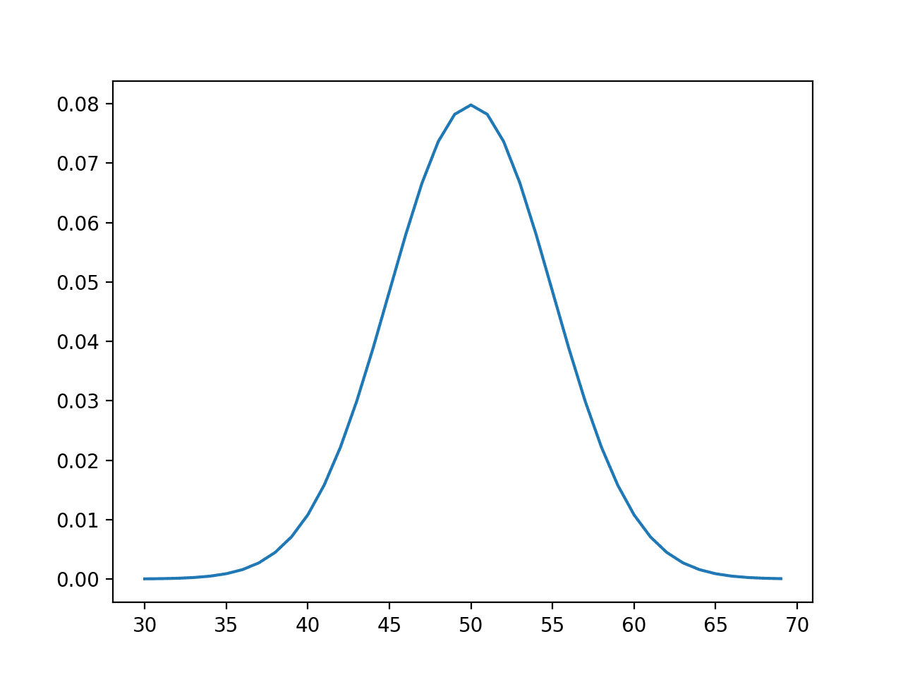
Line Plot of Events vs Probability or the Probability Density Function for the Normal Distribution
The cumulative probabilities are then calculated for observations over the same range, showing that at the mean, we have covered about 50% of the expected values and very close to 100% after the value of about 65 or 3 standard deviations from the mean (50 + (3 * 5)).
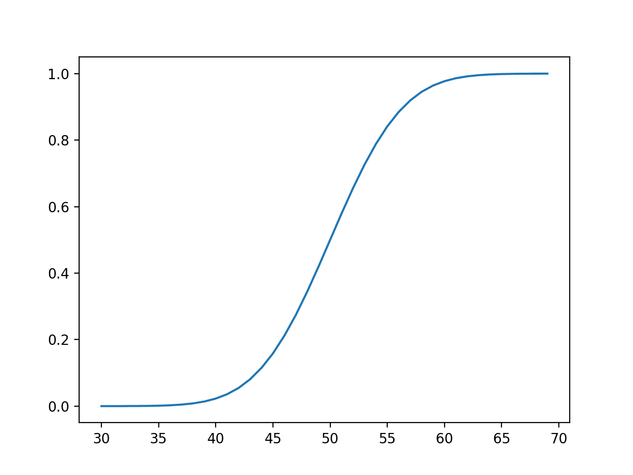
Line Plot of Events vs. Cumulative Probability or the Cumulative Density Function for the Normal Distribution
In fact, the normal distribution has a heuristic or rule of thumb that defines the percentage of data covered by a given range by the number of standard deviations from the mean. It is called the 68-95-99.7 rule, which is the approximate percentage of the data covered by ranges defined by 1, 2, and 3 standard deviations from the mean.
For example, in our distribution with a mean of 50 and a standard deviation of 5, we would expect 95% of the data to be covered by values that are 2 standard deviations from the mean, or 50 – (2 * 5) and 50 + (2 * 5) or between 40 and 60.
We can confirm this by calculating the exact values using the percentage-point function.
The middle 95% would be defined by the percentage point function value for 2.5% at the low end and 97.5% at the high end, where 97.5 – 2.5 gives the middle 95%.
The complete example is listed below.
# calculate the values that define the middle 95%
from scipy.stats import norm
# define distribution parameters
mu = 50
sigma = 5
# create distribution
dist = norm(mu, sigma)
low_end = dist.ppf(0.025)
high_end = dist.ppf(0.975)
print('Middle 95%% between %.1f and %.1f' % (low_end, high_end))
Running the example gives the exact outcomes that define the middle 95% of expected outcomes that are very close to our standard-deviation-based heuristics of 40 and 60.
Middle 95% between 40.2 and 59.8
An important related distribution is the Log-Normal probability distribution.
Exponential Distribution
The exponential distribution is a continuous probability distribution where a few outcomes are the most likely with a rapid decrease in probability to all other outcomes.
It is the continuous random variable equivalent to the geometric probability distribution for discrete random variables.
Some examples of domains that have exponential distribution events include:
- The time between clicks on a Geiger counter.
- The time until the failure of a part.
- The time until the default of a loan.
The distribution can be defined using one parameter:
- Scale (Beta): The mean and standard deviation of the distribution.
Sometimes the distribution is defined more formally with a parameter lambda or rate. The beta parameter is defined as the reciprocal of the lambda parameter (beta = 1/lambda)
- Rate (lambda) = Rate of change in the distribution.
We can define a distribution with a mean of 50 and sample random numbers from this distribution. We can achieve this using the exponential() NumPy function.
The example below samples and prints 10 numbers from this distribution.
# sample an exponential distribution
from numpy.random import exponential
# define the distribution
beta = 50
n = 10
# generate the sample
sample = exponential(beta, n)
print(sample)
Running the example prints 10 numbers randomly sampled from the defined distribution.
[  3.32742946  39.10165624  41.86856606  85.0030387   28.18425491
  68.20434637 106.34826579  19.63637359  17.13805423  15.91135881]
We can define an exponential distribution using the expon() SciPy function and then calculate properties such as the moments, PDF, CDF, and more.
The example below defines a range of observations between 50 and 70 and calculates the probability and cumulative probability for each and plots the result.
# pdf and cdf for an exponential distribution
from scipy.stats import expon
from matplotlib import pyplot
# define distribution parameter
beta = 50
# create distribution
dist = expon(beta)
# plot pdf
values = [value for value in range(50, 70)]
probabilities = [dist.pdf(value) for value in values]
pyplot.plot(values, probabilities)
pyplot.show()
# plot cdf
cprobs = [dist.cdf(value) for value in values]
pyplot.plot(values, cprobs)
pyplot.show()
Running the example first creates a line plot of outcomes versus probabilities, showing a familiar exponential probability distribution shape.

Line Plot of Events vs. Probability or the Probability Density Function for the Exponential Distribution
Next, the cumulative probabilities for each outcome are calculated and graphed as a line plot, showing that after perhaps a value of 55 that almost 100% of the expected values will be observed.
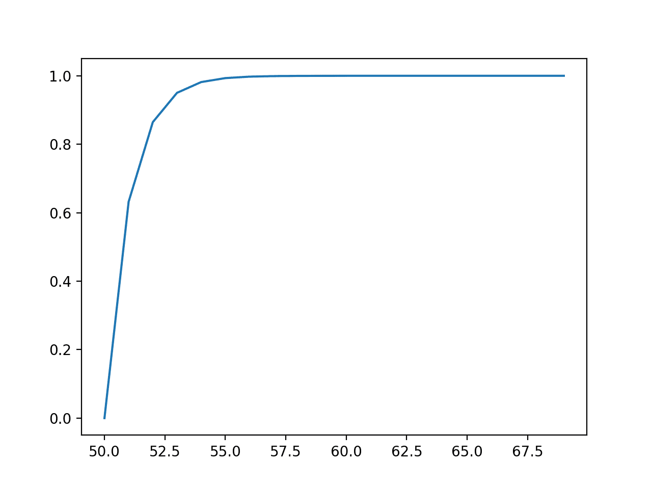
Line Plot of Events vs. Cumulative Probability or the Cumulative Density Function for the Exponential Distribution
An important related distribution is the double exponential distribution, also called the Laplace distribution.
Pareto Distribution
A Pareto distribution is named after Vilfredo Pareto and is may be referred to as a power-law distribution.
It is also related to the Pareto principle (or 80/20 rule) which is a heuristic for continuous random variables that follow a Pareto distribution, where 80% of the events are covered by 20% of the range of outcomes, e.g. most events are drawn from just 20% of the range of the continuous variable.
The Pareto principle is just a heuristic for a specific Pareto distribution, specifically the Pareto Type II distribution, that is perhaps most interesting and on which we will focus.
Some examples of domains that have Pareto distributed events include:
- The income of households in a country.
- The total sales of books.
- The scores by players on a sports team.
The distribution can be defined using one parameter:
- Shape (alpha): The steepness of the decease in probability.
Values for the shape parameter are often small, such as between 1 and 3, with the Pareto principle given when alpha is set to 1.161.
We can define a distribution with a shape of 1.1 and sample random numbers from this distribution. We can achieve this using the pareto() NumPy function.
# sample a pareto distribution
from numpy.random import pareto
# define the distribution
alpha = 1.1
n = 10
# generate the sample
sample = pareto(alpha, n)
print(sample)
Running the example prints 10 numbers randomly sampled from the defined distribution.
[0.5049704  0.0140647  2.13105224 3.10991217 2.87575892 1.06602639
 0.22776379 0.37405415 0.96618778 3.94789299]
We can define a Pareto distribution using the pareto() SciPy function and then calculate properties, such as the moments, PDF, CDF, and more.
The example below defines a range of observations between 1 and about 10 and calculates the probability and cumulative probability for each and plots the result.
# pdf and cdf for a pareto distribution
from scipy.stats import pareto
from matplotlib import pyplot
# define distribution parameter
alpha = 1.5
# create distribution
dist = pareto(alpha)
# plot pdf
values = [value/10.0 for value in range(10, 100)]
probabilities = [dist.pdf(value) for value in values]
pyplot.plot(values, probabilities)
pyplot.show()
# plot cdf
cprobs = [dist.cdf(value) for value in values]
pyplot.plot(values, cprobs)
pyplot.show()
Running the example first creates a line plot of outcomes versus probabilities, showing a familiar Pareto probability distribution shape.
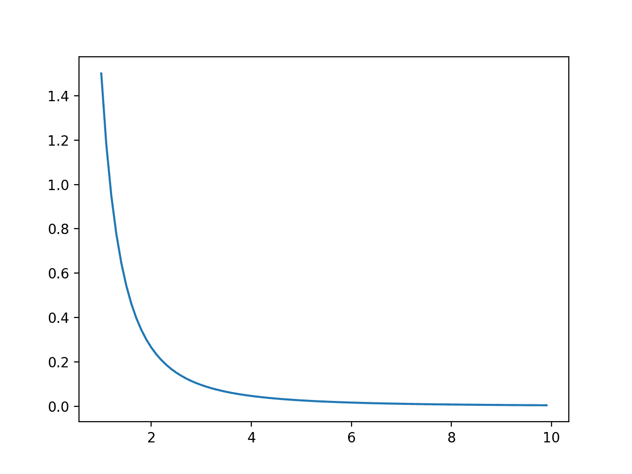
Line Plot of Events vs. Probability or the Probability Density Function for the Pareto Distribution
Next, the cumulative probabilities for each outcome are calculated and graphed as a line plot, showing a rise that is less steep than the exponential distribution seen in the previous section.
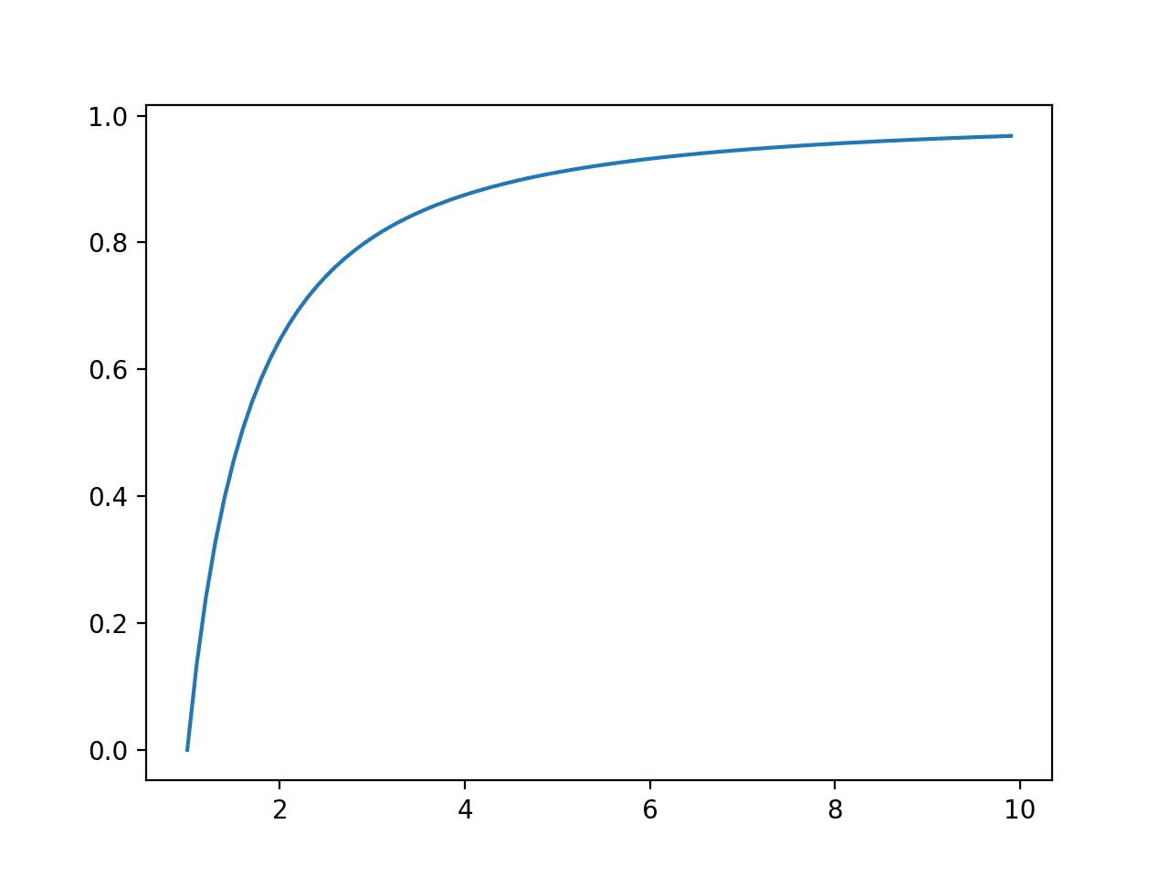
Line Plot of Events vs. Cumulative Probability or the Cumulative Density Function for the Pareto Distribution
Further Reading
This section provides more resources on the topic if you are looking to go deeper.
Books
- Chapter 2: Probability Distributions, Pattern Recognition and Machine Learning, 2006.
- Section 3.9: Common Probability Distributions, Deep Learning, 2016.
- Section 2.3: Some common discrete distributions, Machine Learning: A Probabilistic Perspective, 2012.
API
Articles
- Normal distribution, Wikipedia.
- 68–95–99.7 rule, Wikipedia.
- Exponential distribution, Wikipedia.
- Pareto distribution, Wikipedia.
Summary
In this tutorial, you discovered continuous probability distributions used in machine learning.
Specifically, you learned:
- The probability of outcomes for continuous random variables can be summarized using continuous probability distributions.
- How to parametrize, define, and randomly sample from common continuous probability distributions.
- How to create probability density and cumulative density plots for common continuous probability distributions.
Do you have any questions?
Ask your questions in the comments below and I will do my best to answer.
The post Continuous Probability Distributions for Machine Learning appeared first on Machine Learning Mastery.
Ai
via https://AIupNow.com
Jason Brownlee, Khareem Sudlow
