Last Updated on November 25, 2021
This tutorial is designed for anyone looking for a deeper understanding of how Lagrange multipliers are used in building up the model for support vector machines (SVMs). SVMs were initially designed to solve binary classification problems and later extended and applied to regression and unsupervised learning. They have shown their success in solving many complex machine learning classification problems.
In this tutorial, we’ll look at the simplest SVM that assumes that the positive and negative examples can be completely separated via a linear hyperplane.
After completing this tutorial, you will know:
- How the hyperplane acts as the decision boundary
- Mathematical constraints on the positive and negative examples
- What is the margin and how to maximize the margin
- Role of Lagrange multipliers in maximizing the margin
- How to determine the separating hyperplane for the separable case
Let’s get started.

Method Of Lagrange Multipliers: The Theory Behind Support Vector Machines (Part 1: The separable case)
Photo by Mehreen Saeed, some rights reserved.
This tutorial is divided into three parts; they are:
- Formulation of the mathematical model of SVM
- Solution of finding the maximum margin hyperplane via the method of Lagrange multipliers
- Solved example to demonstrate all concepts
Notations Used In This Tutorial
- $x$: Data point, which is an n-dimensional vector.
- $x^+$: Data point labelled as +1.
- $x^-$: Data point labelled as -1.
- $i$: Subscript used to index the training points.
- $t$: Label of a data point.
- T: Transpose operator.
- $w$: Weight vector denoting the coefficients of the hyperplane. It is also an n-dimensional vector.
- $\alpha$: Lagrange multipliers, one per each training point. This is also an n-dimensional vector.
- $d$: Perpendicular distance of a data point from the decision boundary.
The Hyperplane As The Decision Boundary
The support vector machine is designed to discriminate data points belonging to two different classes. One set of points is labelled as +1 also called the positive class. The other set of points is labeled as -1 also called the negative class. For now, we’ll make a simplifying assumption that points from both classes can be discriminated via linear hyperplane.
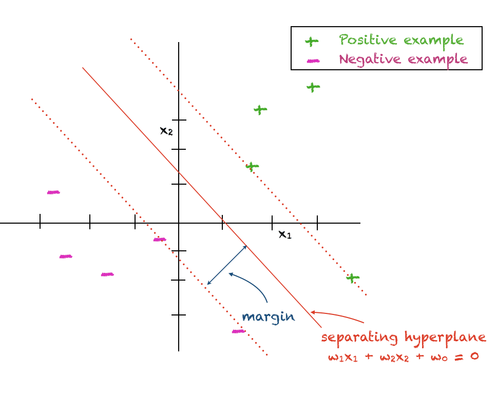
The SVM assumes a linear decision boundary between the two classes and the goal is to find a hyperplane that gives the maximum separation between the two classes. For this reason, the alternate term maximum margin classifier is also sometimes used to refer to an SVM. The perpendicular distance between the closest data point and the decision boundary is referred to as the margin. As the margin completely separates the positive and negative examples and does not tolerate any errors, it is also called the hard margin.
The mathematical expression for a hyperplane is given below with \(w_i\) being the coefficients and \(w_0\) being the arbitrary constant that determines the distance of the hyperplane from the origin:
$$
w^T x_i + w_0 = 0
$$
For the ith 2-dimensional point $(x_{i1}, x_{i2})$ the above expression is reduced to:
$$
w_1x_{i1} + w_2 x_{i2} + w_0 = 0
$$
Mathematical Constraints On Positive and Negative Data Points
As we are looking to maximize the margin between positive and negative data points, we would like the positive data points to satisfy the following constraint:
$$
w^T x_i^+ + w_0 \geq +1
$$
Similarly, the negative data points should satisfy:
$$
w^T x_i^- + w_0 \leq -1
$$
We can use a neat trick to write a uniform equation for both set of points by using $t_i \in \{-1,+1\}$ to denote the class label of data point $x_i$:
$$
t_i(w^T x_i + w_0) \geq +1
$$
The Maximum Margin Hyperplane
The perpendicular distance $d_i$ of a data point $x_i$ from the margin is given by:
$$
d_i = \frac{|w^T x_i + w_0|}{||w||}
$$
To maximize this distance, we can minimize the square of the denominator to give us a quadratic programming problem given by:
$$
\min \frac{1}{2}||w||^2 \;\text{ subject to } t_i(w^Tx_i+w_0) \geq +1, \forall i
$$
Solution Via The Method Of Lagrange Multipliers
To solve the above quadratic programming problem with inequality constraints, we can use the method of Lagrange multipliers. The Lagrange function is therefore:
$$
L(w, w_0, \alpha) = \frac{1}{2}||w||^2 + \sum_i \alpha_i\big(t_i(w^Tx_i+w_0) – 1\big)
$$
To solve the above, we set the following:
\begin{equation}
\frac{\partial L}{ \partial w} = 0, \\
\frac{\partial L}{ \partial \alpha} = 0, \\
\frac{\partial L}{ \partial w_0} = 0 \\
\end{equation}
Plugging above in the Lagrange function gives us the following optimization problem, also called the dual:
$$
L_d = -\frac{1}{2} \sum_i \sum_k \alpha_i \alpha_k t_i t_k (x_i)^T (x_k) + \sum_i \alpha_i
$$
We have to maximize the above subject to the following:
$$
w = \sum_i \alpha_i t_i x_i
$$
and
$$
0=\sum_i \alpha_i t_i
$$
The nice thing about the above is that we have an expression for \(w\) in terms of Lagrange multipliers. The objective function involves no $w$ term. There is a Lagrange multiplier associated with each data point. The computation of $w_0$ is also explained later.
Deciding The Classification of a Test Point
The classification of any test point $x$ can be determined using this expression:
$$
y(x) = \sum_i \alpha_i t_i x^T x_i + w_0
$$
A positive value of $y(x)$ implies $x\in+1$ and a negative value means $x\in-1$
Karush-Kuhn-Tucker Conditions
Also, Karush-Kuhn-Tucker (KKT) conditions are satisfied by the above constrained optimization problem as given by:
\begin{eqnarray}
\alpha_i &\geq& 0 \\
t_i y(x_i) -1 &\geq& 0 \\
\alpha_i(t_i y(x_i) -1) &=& 0
\end{eqnarray}
Interpretation Of KKT Conditions
The KKT conditions dictate that for each data point one of the following is true:
- The Lagrange multiplier is zero, i.e., \(\alpha_i=0\). This point, therefore, plays no role in classification
OR
- $ t_i y(x_i) = 1$ and $\alpha_i > 0$: In this case, the data point has a role in deciding the value of $w$. Such a point is called a support vector.
Computing w_0
For $w_0$, we can select any support vector $x_s$ and solve
$$
t_s y(x_s) = 1
$$
giving us:
$$
t_s(\sum_i \alpha_i t_i x_s^T x_i + w_0) = 1
$$
A Solved Example
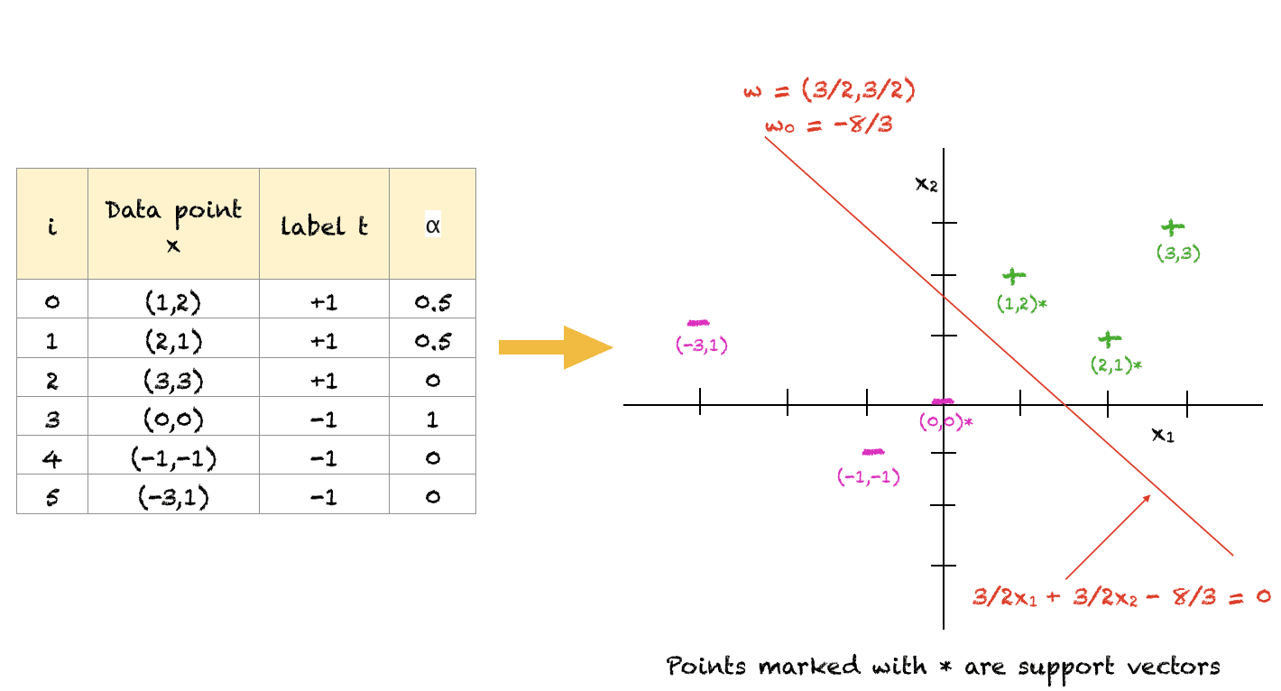
To help you understand the above concepts, here is a simple arbitrarily solved example. Of course, for a large number of points you would use an optimization software to solve this. Also, this is one possible solution that satisfies all the constraints. The objective function can be maximized further but the slope of the hyperplane will remain the same for an optimal solution. Also, for this example, $w_0$ was computed by taking the average of $w_0$ from all three support vectors.
This example will show you that the model is not as complex as it looks.
For the above set of points, we can see that (1,2), (2,1) and (0,0) are points closest to the separating hyperplane and hence, act as support vectors. Points far away from the boundary (e.g. (-3,1)) do not play any role in determining the classification of the points.
Further Reading
This section provides more resources on the topic if you are looking to go deeper.
Books
- Pattern Recognition and Machine Learning by Christopher M. Bishop
- Thomas’ Calculus, 14th edition, 2017 (based on the original works of George B. Thomas, revised by Joel Hass, Christopher Heil, Maurice Weir)
Articles
- Support Vector Machines for Machine Learning
- A Tutorial on Support Vector Machines for Pattern Recognition by Christopher J.C. Burges
Summary
In this tutorial, you discovered how to use the method of Lagrange multipliers to solve the problem of maximizing the margin via a quadratic programming problem with inequality constraints.
Specifically, you learned:
- The mathematical expression for a separating linear hyperplane
- The maximum margin as a solution of a quadratic programming problem with inequality constraint
- How to find a linear hyperplane between positive and negative examples using the method of Lagrange multipliers
Do you have any questions about the SVM discussed in this post? Ask your questions in the comments below and I will do my best to answer.
The post Method Of Lagrange Multipliers: The Theory Behind Support Vector Machines (Part 1: The Separable Case) appeared first on Machine Learning Mastery.
via https://AIupNow.com
Mehreen Saeed, Khareem Sudlow

